timestepping Namespace Reference
Timestepping methods used to solve PDEs in time and space. More...
Classes | |
| class | Alpha |
| Timestep strategy for the Alpha algorithm of Hilber, Hughes and Taylor to solve second order problems in time with no first order time derivative. More... | |
| class | Euler |
| Timestep strategy for the explicit Euler algorithm to solve first order problems in time. More... | |
| class | LimitingEuler |
| Timestep strategy for the explicit Euler algorithm with limiter to solve first order problems in time. More... | |
| class | LimitingTvdRK2 |
| Timestep stategy for an explicit two stage TVD Runge Kutta scheme to solve problems in time. More... | |
| class | Newmark |
| Timestep strategy for the Newmark algorithm to solve second order problems in time with no first order time derivative. More... | |
| class | Nystroem |
| Timestep strategy for a Nyström algorithm to solve second order problems in time with no first order time derivative. More... | |
| class | RungeKutta2 |
| Timestep strategy for the explicit 2nd order RungeKutta algorithm to solve first order problems in time. More... | |
| class | RungeKutta4 |
| Timestep strategy for the explicit 4th order RungeKutta algorithm to solve first order problems in time. More... | |
| class | Theta |
| Timestep strategy for the Theta-Scheme algorithm for first order problems in time. More... | |
| class | TimeLinearForm |
| Abstract class implementing time dependent linear forms. More... | |
| class | TimeStepping |
| This class encapsulates a general timestep solver concept to solve linear PDE in time and space. More... | |
| class | TimeStepStrategy |
| Abstract strategy class for the class Timestepping. More... | |
| class | TimeVector |
| Class implementing time dependent vectors. More... | |
| class | TvdRK2 |
| Timestep stategy for an explicit two stage TVD Runge Kutta scheme to solve problems in time. More... | |
Detailed Description
Timestepping methods used to solve PDEs in time and space.
The discretisation in space is done by the others parts of the library, the discretisation in time is done by this part of the library.
// Space
Line msh;
concepts::BoundaryConditions bc;
linearFEM::Linear1d spc(msh, 4, bc.get());
// Space operators
Laplace stiff_bf;
concepts::SparseMatrix<Real> stiff(spc, stiff_bf);
Identity mass_bf(gauss_p);
concepts::SparseMatrix<Real> mass(spc, mass_bf);
// Zero initial conditions
concepts::Vector<Real> initial(spc)
concepts::Vector<Real> d_dt_initial(spc)
// External driver
Sin_tlf driver_tlf(1.0, 1.0 , 0.0, 0.0, 1);
timestepping::TimeVector driver(spc, driver_tlf);
// Strategy and Solver
timestepping::Newmark timeStepStrategy(mass, stiff, driver, initial,
                                       d_dt_initial, 0.01);
concepts::SuperLUFabric<> fabric;
timestepping::TimeStepping solver(timeStepStrategy, fabric);
// Write solutions to file in Gnuplot format
for(uint n = 0; n <= 5; ++n) {
  solver(sol, n*100/5);
  std::strstream filename;
  filename << "gnuplot/sol1d-" << n << ".gnuplot" << std::ends;
  graphics::DataGnuplot(spc, filename.str(), sol);
}
The follwing picture illustrates the wave equation solved on a rope.
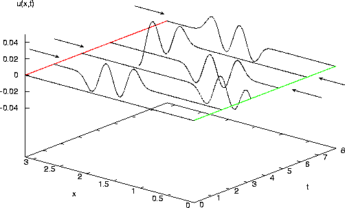
The red line indicates Neumann boundary conditions and the green line Dirichlet boundary conditions. The arrows point in the direction of the movent of the waves. One can clearly see the the waves are reflected on the boundaries and that they do change sign on the Dirichlet boundary and do not change sign on the Neumann boundary.
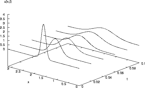
The next picture illustrates the heat equation solved on a wand: the intial peak flattens out as the heat dissipates. Boundary conditions are homogenous Dirichlet.