linearFEM1d.cc

Introduction

One dimensional FEM in Concepts. This code features first order Ansatz functions on a (possibly) uniformly refined mesh.

The equation solved is

-u''+u = x²

on (-1,1) with homogeneous Dirichlet boundary conditions. The linear system is solved using CG.

The exact solution is u = -3 cosh(x)/cosh(1) + x^2 + 2.

The convergence of the relative energy error and the maximal nodal error are shown together with plots of the solution.

Contents

1. Commented Program
   1. Mesh
   2. FEM Routine
   3. Main Program
2. Results
3. Complete Source Code

Commented Program

System include files. The first is for input and output operations, the second one declares unique_ptr and the third is for stringstream.

#include <iostream>
#include <memory>
#include <sstream>
#include <unistd.h> // for command line parsing

Concepts include files.

#include "basics.hh"
#include "geometry.hh"
#include "space.hh"
#include "toolbox.hh"
#include "function.hh"
#include "operator.hh"
#include "integration.hh"
#include "graphics.hh"
#include "linearFEM.hh"

With this using directive, we do not need to prepend concepts:: before Real everytime.

using concepts::Real;

Mesh

The mesh is taken from the meshes tutorial: Line. Here, the relevant code is included:

#include "meshes.cc"

Linear Form

The linear form is used to compute the element contributions to the load vector. The computations are done in the application operator of this class.

class RHS : public concepts::LinearForm<Real> {
private:

As we need numerical integration, the class has a member quad_ of type concepts::Quadrature. The template parameter 4 indicates the type of quadrature rule. It contains the quadrature points and weights for given number of quadrature points (gauss_p).

The constructor takes as argument the number of quadrature points gauss_p and initialises the quadrature object quad_.

  const concepts::Quadrature<4> quad_;
public:
  RHS(const uint gauss_p = 1) : quad_(gauss_p) {}

The application operator is called for every element elm and is responsible for computing the contributions of this element to the global load vector. The local load vector is stored in em.

  virtual void operator()(const concepts::Element<Real>& elm,
        concepts::ElementMatrix<Real>& em) const {

Resize the element load vector to the correct size and set all entries to zero. This way, the computed values can be added into em.

    const uint n = elm.T().m();
    em.resize(n, 1);
    em.zeros();

Check if the general element elm really is an element of type linearFEM::Line which can be handled by our routine. This is achieved by trying to cast elm to linearFEM::Line. If the cast succeeds (ie. elm is really of type linearFEM::Line), then e contains a pointer to this element. If the cast fails, e is equal to 0 and the assertion fails too. If the assertions fails, an error message is displayed (indicating the name of the file, the line number in the file, the name of the routine where the error happened and the check which failed) and the execution of the program stops.

    const linearFEM::Line* e = dynamic_cast<const linearFEM::Line*>(&elm);
    conceptsAssert(e, concepts::Assertion());

The element of type linearFEM::Line has a member cell which returns a reference to a concepts::Edge1d and this class is able to compute the size of the cell (on which the element is based). The size of the cell is needed to compute the Jacobian in the numerical integration.

    const Real h = e->cell().size();

Next, we get pointers to the first elements of the arrays of quadrature weights and points. These data were computed in the constructor (which initialised the member quad_).

    const Real* w = quad_.weights();   // quadrature weights
    const Real* q = quad_.abscissas(); // quadrature points

Now, the computational loops of this routine start.

There are two nested loops here: the outer loop enumerates the shape funtions of this element and the inner loop enumerates the quadrature points.

    for (uint i = 0; i < n; ++i) { // loop over shape functions

m is a reference to the entry of the local load vector which corresponds to the current shape function.

      Real& m = em(i,0);
      for (uint k = 0; k < quad_.n(); ++k) { // loop over quadrature points

Now, all data is known to add to m:

• w[k] is the quadrature weight associated to the current quadrature point q[k].

    m += w[k]

• h is the determinant of the Jacobian of the element map which maps the reference coordinates (0,1) to the physical coordinates of this element. 1/2 is the Jacobian of the map from (-1,1) to (0,1). The integration takes place on (-1,1) (as described in concepts::Quadrature).

      * h / 2.0

• e->shapefct(i, q[k]) is the value of the shape function i at the point q[k]. As you can see in linearFEM::Line, it takes values in (-1,1).

      * e->shapefct(i, q[k])

• The last line pow(e->cell().chi( (1.0+q[k])/2.0 ), 2.0) computes the value of the right hand side funtion f = x². (1.0+q[k])/2.0 maps a point in (-1,1) to (0,1) and the function pow from the standard math library computes a^b.

      * pow(e->cell().chi( (1.0+q[k])/2.0 ), 2.0);
        } // for k
      } // for i
    }
  };

The exact solution.

Real exact(const Real x) {
  return -3.0*cosh(x)/cosh(1.0)+x*x+2.0;
}

FEM Routine

The only parameters of the routine fem are the maximal level of refinement and the number of quadrature points. The additional argument output is used to for the gathering the output.

void fem(const uint level, const uint gauss_p,
   concepts::InOutParameters& output) {

Set up the mesh. The values -1, 0 and 1 give the coordinates of the left, middle and right points in the mesh.

  Line msh(-1, 0, 1);
  std::cout << "Mesh: " << msh << std::endl;

The boundary conditions are given by assigning a boundary type to an attribute. The end points of the interval which are created above have the attribute 2.

The class Boundary holds a type (Dirichlet or Neumann) and (if necessary) a function or value. These objects can be added to BoundaryConditions which manages them.

  concepts::BoundaryConditions bc;
  bc.add(concepts::Attribute(2),
   concepts::Boundary(concepts::Boundary::DIRICHLET));
  std::cout << "Boundary conditions: " << bc << std::endl;

Start the loop over the different levels.

  for (uint l = 1; l < level; ++l) {
    std::cout << "l = " << l << std::endl;

Set up the space according to the current level. The space takes the mesh, the level of refinement and the boundary conditions as input. If there are Dirichlet boundary conditions somewhere, the respective degrees of freedom are not created.

    linearFEM::Linear1d spc(msh, l, &bc);
    std::cout << "Space: " << spc << std::endl;

Compute the load vector. This is done by creating an object of type RHS which is a linear form. This linear form is then given to the vector. The vector fills its entries by evaluating the linear form on every element of the space and assembling the local load vectors according to the assembling information contained in the elements.

    RHS rhs_lf(gauss_p);
    concepts::Vector<Real> rhs(spc, rhs_lf);

Compute the stiffness matrix and the mass matrix. As above, a bilinear form is created and given to a matrix which the assembles the mass and stiffness matrix respectively.

    linearFEM::Laplace1d stiff_bf;
    concepts::SparseMatrix<Real> stiff(spc, stiff_bf);
 
    linearFEM::Identity1d mass_bf;
    concepts::SparseMatrix<Real> mass(spc, mass_bf);

A linear combination L is formed from the mass and stiffness matrix. The linear system is going to be solved iteratively. This linear combination is used to initialize a CG solver together with the maximal residual and the maximal number of iterations.

    concepts::LiCo<Real> L(stiff, mass, 1.0, 1.0);
    concepts::CG<Real> solver(L, 1e-6, 2000);

An empty vector to hold the solution of the linear system.

    concepts::Vector<Real> sol(spc);
    try {

The CG solver is essentially a linear operator. Therefore, one can apply a vector to it and get the solution of the linear system which was used to set up the CG solver.

      solver(rhs, sol);
    }

The CG solver throws a exception of type concepts::NoConvergence which is caught here. Although the solver might not have converged, the solution might give some hints to the user. Therefore, the execution of the program is not stopped here and only a warning message is displayed.

    catch(concepts::NoConvergence& e) {
      std::cout << "solver did not converge!" << std::endl << e << std::endl;
    }

Print some information about the solution process and the solution itself.

    std::cout << "solver = " << solver << std::endl;
    std::cout << "solution = " << sol << std::endl;

Gather the results of the computation. Using output, all data can be displayed and/or saved at the end.

• mesh size h

      const Real h = 1.0/(1<<l);
      output.addArrayDouble("h", l, h);

• maximal nodal error

      Real x = -1.0;
      Real maxNodalFehler = 0.0;
      Real nodalFehler = 0.0;
      for (uint p = 0; p < spc.dim(); ++p, x += h) {
        nodalFehler = fabs(sol[p] - exact(x));
        if (nodalFehler > maxNodalFehler)
    maxNodalFehler = nodalFehler;
      }
      output.addArrayDouble("maxNodalFehler", l, maxNodalFehler);

• FE energy error

      const Real exEnergie = output.getDouble("exEnergie");
      const Real feEnergie(sol*rhs);
      output.addArrayDouble("energieFehler", l,
          fabs(exEnergie-feEnergie)/exEnergie);

Last but not least, the solution vector is stored in a text file suitable for Gnuplot. See the results section on how to process this file.

    std::stringstream filename;
    filename << "solution1d-" << l << ".gnuplot" << std::ends;

End of the loop over the different levels.

    graphics::drawDataGnuplot(spc, filename.str(), sol);
  } // for l
}

Main Program

The main program just does some comand line parameter handling calls the main function fem. It also features the main try...catch brace to catch exceptions thrown by the program.

int main(int argc, char** argv) {
 
  try {

The inputParser takes care of all input parameters and the results which are gathered (see input output tutorial). At the end, they can be printed.

    concepts::InputParser inputParser(true);
    concepts::InOutParameters& input = inputParser.inputParameters();

Default values for the variable which could be set by a command line argument: the maximal level of refinement and the number of points for the Gauss quadrature.

    input.addInt("level", 1);
    input.addInt("gauss_p", 1);

Parse the command line options using the standard library method getopt. Have a look at getopt(3) to find out more about this function.

    int opt;
    while ((opt = getopt(argc, argv, "-l:p:")) != EOF)
      switch(opt) {
      case 'l': input.addInt("level", std::atoi(optarg)); break;
      case 'p': input.addInt("gauss_p", std::atoi(optarg)); break;
      default:
  std::cout << "Usage: " << argv[0] 
      << " [-l LEVEL] [-p GAUSS_P]" << std::endl
      << "where" << std::endl
      << "  LEVEL: maximal level of refinement" << std::endl
      << "  GAUSS_P: number of points in Gauss integration"
      << std::endl;
  std::exit(1); break;
      }

Prepare the results part to gather the results and compute the exact FE energy and the element size.

    concepts::InOutParameters& output = inputParser.outputParameters();
    const Real exEnergie = 206.0/15.0
      + 36.0*exp(2.0)/(exp(2.0)+1.0)/(exp(2.0)+1.0)*sinh(2.0)
      - 72.0*exp(1.0)/(exp(2.0)+1.0)*sinh(1.0);
    output.addDouble("exEnergie", exEnergie);
    output.addArrayDouble("h");
    output.addArrayDouble("energieFehler");
    output.addArrayDouble("maxNodalFehler");

The values for the level and the quadrature points are fixed now, call fem.

    fem(input.getInt("level"), input.getInt("gauss_p"), output);

Print the results.

    std::cout << inputParser << std::endl;

In order to be able to plot the numbers computed in the fem routine, it is convenient to have them in table suitable for Gnuplot.

    concepts::ResultsTable table;

Every array from output which should be present in the table has to be added to table.

    table.addMap(concepts::ResultsTable::DOUBLE, "h", output);
    table.addMap(concepts::ResultsTable::DOUBLE, "energieFehler", output);
    table.addMap(concepts::ResultsTable::DOUBLE, "maxNodalFehler", output);

Then, a file is created with high numerical output precision and the table is printed to the file. The file is closed automatically. See the results section on how to process this file.

    std::ofstream ofs("linearFEM1d.gnuplot");
    ofs << std::setprecision(20);
    table.print<concepts::ResultsTable::GNUPLOT>(ofs);
  }

Here, the exceptions are caught and some output is generated. Normally, this should not happen.

  catch(concepts::ExceptionBase& e) {
    std::cout << e << std::endl;
    return 1;
  }

Sane return value.

  return 0;
}

Results

Output of the program:

$ linearFEM1d -l 3
Mesh: Line(Edge1d(idx = (0, 0), cntr = Edge(Key(0), (Vertex(Key(0)), Vertex(Key(1))), Attribute(0)), vtx = [-1, 0], map = MapEdge1d(-1, 0)),
Edge1d(idx = (0, 0), cntr = Edge(Key(1), (Vertex(Key(1)), Vertex(Key(2))), Attribute(0)), vtx = [0, 1], map = MapEdge1d(0, 1)))
Boundary conditions: BoundaryConditions(2: Boundary(DIRICHLET, (0)), 0: Boundary(FREE, (0)))
l = 1
Space: Linear1d(dim = 3, nelm = 4)
solver = CG(solves LiCo(1 * SparseMatrix(3x3, HashedSparseMatrix: 7 (77.7778%) entries bound.) + 1 * SparseMatrix(3x3, HashedSparseMatrix: 7 (77.7778%) entries bound.)), eps = 9.5313e-34, it = 2, relres = 0)
solution = Vector(3, [0.0644745, 0.0642467, 0.0644745])
l = 2
Space: Linear1d(dim = 7, nelm = 8)
solver = CG(solves LiCo(1 * SparseMatrix(7x7, HashedSparseMatrix: 19 (38.7755%) entries bound.) + 1 * SparseMatrix(7x7, HashedSparseMatrix: 19 (38.7755%) entries bound.)), eps = 1.01691e-33, it = 4, relres = 0)
solution = Vector(7, [0.0464661, 0.0593538, 0.0592139, 0.0578795, 0.0592139, 0.0593538, 0.0464661])
/* time, date:  Mon Jan 27 15:00:05 2003
 * username:    pfrauenf
 * sysname:     Linux
 * nodename:    herodot
 * release:     2.4.18
 * version:     2.4.18
 * machine:     i686
 */
string  author  "(empty)"
string  comment "(empty)"
string  title   "(empty)"
int     gauss_p 1
int     level   3
end
// output starts here
double  exEnergie       0.0246385
array double energieFehler {
        1       0.100759
        2       0.0318543
}
array double h {
        1       0.5
        2       0.25
}
array double maxNodalFehler {
        1       0.0644745
        2       0.0464661
} 

Error diagrams:
<img src="linearFEM1d-conv.png" width="640" height="480" alt="error diagram">
The diagram above was created using the following commands: @code

set logscale x set logscale y set grid set grid mxtics set grid mytics set key top left set xlabel 'h' set ylabel 'error' plot 'linearFEM1d-1.gnuplot' using 3:2 title 'relative energy error, gauss_p = 1', \ '' using 3:4 title 'max nodal error, gauss_p = 1', \ 'linearFEM1d-2.gnuplot' using 3:2 title 'relative energy error, gauss_p = 2', \ '' using 3:4 title 'max nodal error, gauss_p = 2'

Exact and numerical solution: 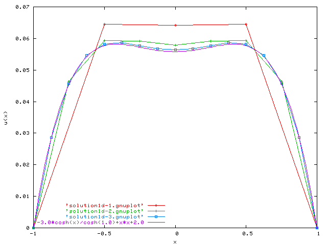The diagram above was created using the following commands:

set xlabel 'x'
set ylabel 'u(x)'
set key bottom left
plot 'solution1d-1.gnuplot', 'solution1d-2.gnuplot', 'solution1d-3.gnuplot', -3.0*cosh(x)/cosh(1.0)+x*x+2.0 

@section complete Complete Source Code
@author Philipp Frauenfelder, 2004

#include <iostream>
#include <memory>
#include <sstream>
#include <unistd.h> // for command line parsing
 
#include "basics.hh"
#include "geometry.hh"
#include "space.hh"
#include "toolbox.hh"
#include "function.hh"
#include "operator.hh"
#include "integration.hh"
#include "graphics.hh"
#include "linearFEM.hh"
 
using concepts::Real;
 
#include "meshes.cc"
 
// ************************************************************* Linear Form **
 
class RHS : public concepts::LinearForm<Real> {
private:
  const concepts::Quadrature<4> quad_;
public:
  RHS(const uint gauss_p = 1) : quad_(gauss_p) {}
 
  virtual void operator()(const concepts::Element<Real>& elm,
        concepts::ElementMatrix<Real>& em) const {
    const uint n = elm.T().m();
    em.resize(n, 1);
    em.zeros();
 
    const linearFEM::Line* e = dynamic_cast<const linearFEM::Line*>(&elm);
    conceptsAssert(e, concepts::Assertion());
 
    const Real h = e->cell().size();
    const Real* w = quad_.weights();   // quadrature weights
    const Real* q = quad_.abscissas(); // quadrature points
 
    for (uint i = 0; i < n; ++i) { // loop over shape functions
      Real& m = em(i,0);
      for (uint k = 0; k < quad_.n(); ++k) { // loop over quadrature points
  m += w[k]
    * h / 2.0
    * e->shapefct(i, q[k])
    * pow(e->cell().chi( (1.0+q[k])/2.0 ), 2.0);
      } // for k
    } // for i
  }
};
 
Real exact(const Real x) {
  return -3.0*cosh(x)/cosh(1.0)+x*x+2.0;
}
 
void fem(const uint level, const uint gauss_p,
   concepts::InOutParameters& output) {
  Line msh(-1, 0, 1);
  std::cout << "Mesh: " << msh << std::endl;
 
  concepts::BoundaryConditions bc;
  bc.add(concepts::Attribute(2),
   concepts::Boundary(concepts::Boundary::DIRICHLET));
  std::cout << "Boundary conditions: " << bc << std::endl;
 
  for (uint l = 1; l < level; ++l) {
    std::cout << "l = " << l << std::endl;
 
    linearFEM::Linear1d spc(msh, l, &bc);
    std::cout << "Space: " << spc << std::endl;
 
    RHS rhs_lf(gauss_p);
    concepts::Vector<Real> rhs(spc, rhs_lf);
 
    linearFEM::Laplace1d stiff_bf;
    concepts::SparseMatrix<Real> stiff(spc, stiff_bf);
 
    linearFEM::Identity1d mass_bf;
    concepts::SparseMatrix<Real> mass(spc, mass_bf);
 
    concepts::LiCo<Real> L(stiff, mass, 1.0, 1.0);
    concepts::CG<Real> solver(L, 1e-6, 2000);
 
    concepts::Vector<Real> sol(spc);
    try {
      solver(rhs, sol);
    }
    catch(concepts::NoConvergence& e) {
      std::cout << "solver did not converge!" << std::endl << e << std::endl;
    }
    std::cout << "solver = " << solver << std::endl;
    std::cout << "solution = " << sol << std::endl;
 
    const Real h = 1.0/(1<<l);
    output.addArrayDouble("h", l, h);
 
    Real x = -1.0;
    Real maxNodalFehler = 0.0;
    Real nodalFehler = 0.0;
    for (uint p = 0; p < spc.dim(); ++p, x += h) {
      nodalFehler = fabs(sol[p] - exact(x));
      if (nodalFehler > maxNodalFehler)
  maxNodalFehler = nodalFehler;
    }
    output.addArrayDouble("maxNodalFehler", l, maxNodalFehler);
 
    const Real exEnergie = output.getDouble("exEnergie");
    const Real feEnergie(sol*rhs);
    output.addArrayDouble("energieFehler", l,
        fabs(exEnergie-feEnergie)/exEnergie);
 
    std::stringstream filename;
    filename << "solution1d-" << l << ".gnuplot" << std::ends;
    graphics::drawDataGnuplot(spc, filename.str(), sol);
  } // for l
}
 
// ************************************************************ Main Program **
 
int main(int argc, char** argv) {
 
  try {
    concepts::InputParser inputParser(true);
    concepts::InOutParameters& input = inputParser.inputParameters();
    input.addInt("level", 1);
    input.addInt("gauss_p", 1);
 
    int opt;
    while ((opt = getopt(argc, argv, "-l:p:")) != EOF)
      switch(opt) {
      case 'l': input.addInt("level", std::atoi(optarg)); break;
      case 'p': input.addInt("gauss_p", std::atoi(optarg)); break;
      default:
  std::cout << "Usage: " << argv[0] 
      << " [-l LEVEL] [-p GAUSS_P]" << std::endl
      << "where" << std::endl
      << "  LEVEL: maximal level of refinement" << std::endl
      << "  GAUSS_P: number of points in Gauss integration"
      << std::endl;
  std::exit(1); break;
      }
 
    concepts::InOutParameters& output = inputParser.outputParameters();
    const Real exEnergie = 206.0/15.0
      + 36.0*exp(2.0)/(exp(2.0)+1.0)/(exp(2.0)+1.0)*sinh(2.0)
      - 72.0*exp(1.0)/(exp(2.0)+1.0)*sinh(1.0);
    output.addDouble("exEnergie", exEnergie);
    output.addArrayDouble("h");
    output.addArrayDouble("energieFehler");
    output.addArrayDouble("maxNodalFehler");
 
    fem(input.getInt("level"), input.getInt("gauss_p"), output);
 
    std::cout << inputParser << std::endl;
 
    concepts::ResultsTable table;
    table.addMap(concepts::ResultsTable::DOUBLE, "h", output);
    table.addMap(concepts::ResultsTable::DOUBLE, "energieFehler", output);
    table.addMap(concepts::ResultsTable::DOUBLE, "maxNodalFehler", output);
    std::ofstream ofs("linearFEM1d.gnuplot");
    ofs << std::setprecision(20);
    table.print<concepts::ResultsTable::GNUPLOT>(ofs);
  }
  catch(concepts::ExceptionBase& e) {
    std::cout << e << std::endl;
    return 1;
  }
  return 0;
}