In this tutorial the implementation of Robin boundary conditions using trace spaces is shown.
Now we derive the corresponding variational formulation of the introduced problem: find  such that
are included. With the following using directive
The mesh is read from three files containing the coordinates, the elements and the boundary attributes of the mesh.
In our example the edges are given the following attributes: 1 (bottom), 2 (right), 3 (top) and 4 (left).
Now the mesh is plotted using a scaling factor of 100, a greyscale of 1.0 and one point per edge.
Since we do not have any homogeneous Dirichlet boundary conditions we do not need to set them using concepts::BoundaryConditions bc.
and a set of unsigned intergers identifying the edge with attribute 1, on which the Neumann boundary condition is prescribed, is created.
Now the same is done for the Robin data. The two formulas are defined
and a set of unsigned intergers identifying the edge with attributes 2, 3 and 4, on which the Robin boundary condition is prescribed, is created.
In this example there are no homogeneous Dirichlet boundary conditions and thus, the space can be built without passing any boundary data. We refine the space two times and set the polynomial degree to three. Then the elements of the space are built and the space is plotted.
The right hand side is computed. In our case, the vector rhs only contains the integrals of the Neumann and Robin trace as the source term is zero.
Furthermore, the integrals of the Robin trace are added.
We solve the equation using the conjugate gradient method with a tolerance of 1e-6 and a maximum number of iterations of 200.
Finally, exceptions are caught and a sane return value is given back.
Mesh: Import2dMesh(ncell = 1)
RHS Vector:
Vector(169, [ 1.549354e-02, 1.678744e-01, 0.000000e+00, -9.444769e-02, 1.570060e-02, 5.980456e-03, 0.000000e+00, 0.000000e+00, 0.000000e+00, 0.000000e+00, -8.097468e-03, -3.200783e-03, 0.000000e+00, 0.000000e+00, 0.000000e+00, 0.000000e+00, 2.374103e-01, 0.000000e+00, 3.790460e-02, 2.477186e-03, 0.000000e+00, 0.000000e+00, 0.000000e+00, 0.000000e+00, 0.000000e+00, 0.000000e+00, 0.000000e+00, 0.000000e+00, 0.000000e+00, 0.000000e+00, 0.000000e+00, 0.000000e+00, 0.000000e+00, 0.000000e+00, 0.000000e+00, 0.000000e+00, 0.000000e+00, 0.000000e+00, 0.000000e+00, 0.000000e+00, -1.745166e-01, 0.000000e+00, 0.000000e+00, -2.305964e-02, -2.713493e-03, 0.000000e+00, 0.000000e+00, 0.000000e+00, 0.000000e+00, 1.678744e-01, 0.000000e+00, 3.790460e-02, -2.477186e-03, 0.000000e+00, 0.000000e+00, 0.000000e+00, 0.000000e+00, 0.000000e+00, 0.000000e+00, 0.000000e+00, 0.000000e+00, 1.549354e-02, -9.444769e-02, 1.570060e-02, -5.980456e-03, -8.097468e-03, -3.200783e-03, 0.000000e+00, 0.000000e+00, 0.000000e+00, 0.000000e+00, 0.000000e+00, 0.000000e+00, -1.745166e-01, 0.000000e+00, -2.305964e-02, -2.713493e-03, 0.000000e+00, 0.000000e+00, 0.000000e+00, 0.000000e+00, 0.000000e+00, 0.000000e+00, 0.000000e+00, 0.000000e+00, 0.000000e+00, 0.000000e+00, 0.000000e+00, 0.000000e+00, 0.000000e+00, 0.000000e+00, 0.000000e+00, 0.000000e+00, 0.000000e+00, 0.000000e+00, 0.000000e+00, 0.000000e+00, 0.000000e+00, 0.000000e+00, 0.000000e+00, 0.000000e+00, 0.000000e+00, 0.000000e+00, -2.280169e-01, -3.451119e-02, -1.813098e-03, 0.000000e+00, 0.000000e+00, 0.000000e+00, 0.000000e+00, 0.000000e+00, 0.000000e+00, -2.484019e-01, -2.500000e-01, -4.070872e-02, -6.366754e-04, -4.166667e-02, 1.734723e-18, 0.000000e+00, 0.000000e+00, 0.000000e+00, 0.000000e+00, 0.000000e+00, 0.000000e+00, -2.500000e-01, -4.166667e-02, 1.734723e-18, 0.000000e+00, 0.000000e+00, 0.000000e+00, 0.000000e+00, 0.000000e+00, 0.000000e+00, 0.000000e+00, -2.280169e-01, 0.000000e+00, 0.000000e+00, 0.000000e+00, 0.000000e+00, -3.451119e-02, -1.813098e-03, 0.000000e+00, 0.000000e+00, 0.000000e+00, 0.000000e+00, 0.000000e+00, 0.000000e+00, 0.000000e+00, 0.000000e+00, 0.000000e+00, 0.000000e+00, -2.500000e-01, -4.166667e-02, 1.734723e-18, 0.000000e+00, 0.000000e+00, 0.000000e+00, 0.000000e+00, 0.000000e+00, 0.000000e+00, -2.484019e-01, -4.166667e-02, 1.734723e-18, -4.070872e-02, -6.366754e-04, 0.000000e+00, 0.000000e+00, 0.000000e+00, 0.000000e+00])
System Matrix:
SparseMatrix(169x169, HashedSparseMatrix: 2825 (9.891110e+00%) entries bound.)
Solver:
CG(solves SparseMatrix(169x169, HashedSparseMatrix: 2825 (9.891110e+00%) entries bound.), eps = 2.020060e-13, it = 80, relres = 0)
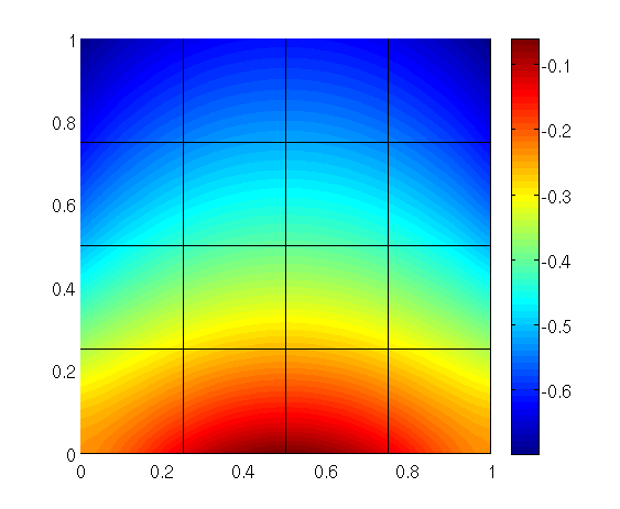
Solution:
Vector(169, [-2.358621e-01, -1.292236e-01, -2.897387e-01, -3.566354e-01, -4.559784e-02, 1.946268e-02, -1.205115e-02, 1.041007e-03, 7.643942e-03, 1.495624e-03, 6.444425e-02, -1.673150e-02, 1.587649e-03, 1.516131e-02, -1.737078e-02, 2.614680e-04, -6.104150e-02, -2.594241e-01, 6.267788e-02, 3.415305e-03, -4.265880e-02, 3.940668e-03, 2.834395e-02, -1.218784e-03, -3.113244e-02, 3.435106e-03, 4.747729e-04, -5.287489e-04, -4.024240e-01, -4.285121e-01, -1.755820e-02, 8.663324e-04, 2.607719e-02, -8.180827e-06, -1.171876e-02, 3.220957e-04, -4.655572e-03, 1.149243e-03, -7.664004e-04, 4.331508e-05, -5.093568e-01, 3.010054e-02, -9.187840e-04, -1.329112e-02, -1.955238e-03, 1.487914e-02, -1.465611e-03, -2.471166e-03, 6.547792e-04, -1.292236e-01, -2.897387e-01, 6.267788e-02, -3.415305e-03, -1.205113e-02, 1.040996e-03, 2.834395e-02, -1.218785e-03, -3.113244e-02, 3.435105e-03, -4.747728e-04, 5.287486e-04, -2.358622e-01, -3.566353e-01, -4.559785e-02, -1.946269e-02, 6.444424e-02, -1.673150e-02, 7.643955e-03, 1.495610e-03, 1.587650e-03, 1.516131e-02, 1.737078e-02, -2.614670e-04, -5.093567e-01, -4.285121e-01, -1.329111e-02, -1.955238e-03, 3.010056e-02, -9.187924e-04, -1.171876e-02, 3.220940e-04, 1.487914e-02, -1.465611e-03, 2.471168e-03, -6.547794e-04, 2.607719e-02, -8.184208e-06, -4.655572e-03, 1.149243e-03, 7.664006e-04, -4.331492e-05, -5.422842e-01, -5.175790e-01, -1.233271e-02, 2.673123e-04, 2.503141e-02, 2.062220e-04, -1.092907e-02, -4.406529e-04, 1.897520e-03, 1.259827e-04, 3.070159e-04, -2.411602e-05, -6.223888e-01, -2.309603e-02, 9.144676e-05, 3.166487e-02, -1.023908e-03, 7.914136e-03, -6.405805e-05, 5.635018e-04, 6.261481e-05, -6.986328e-01, -6.372162e-01, -1.000691e-02, 2.816808e-03, 1.919979e-02, 1.070780e-03, -5.661673e-03, -7.812417e-04, 4.554296e-03, -2.152115e-03, 2.307448e-03, 7.109204e-06, -6.168267e-01, 2.056493e-02, -1.138131e-04, -4.696031e-03, -6.020063e-04, 8.646241e-04, -2.627329e-04, -8.207371e-05, -8.849003e-05, -5.422842e-01, -6.223888e-01, -1.233271e-02, 2.673136e-04, 3.166486e-02, -1.023899e-03, -2.309604e-02, 9.144808e-05, 7.914135e-03, -6.405777e-05, -5.635004e-04, -6.261480e-05, 2.503142e-02, 2.062226e-04, 1.897520e-03, 1.259829e-04, -3.070157e-04, 2.411587e-05, -6.372162e-01, 2.056493e-02, 1.138135e-04, -5.661684e-03, -7.812348e-04, 8.646239e-04, -2.627334e-04, 8.207376e-05, 8.849023e-05, -6.986327e-01, 1.919980e-02, -1.070775e-03, -1.000690e-02, 2.816814e-03, 4.554296e-03, -2.152114e-03, -2.307448e-03, -7.109961e-06])
![\[ - \Delta u + u = 0 \]](form_185.png)
 with inhomogeneous Neumann boundary condition
 ![\[ \nabla u\cdot \underline{n} = g(x,y), \qquad (x,y)\in\Gamma_{\rm N}=\{(x,y)\in\partial\Omega\mid y=0\}, \]](form_187.png)
![\[ \nabla u\cdot \underline{n} = h_1(x,y) u + h_2(x,y), \qquad (x,y)\in\Gamma_{\rm R}=\partial\Omega\setminus\Gamma_{\rm N} \]](form_202.png)
 ,
,  and
and  .
.![\[ \int_{\Omega} \nabla u \cdot \nabla v \;{\rm d}x + \int_{\Omega} u v \;{\rm d}x - \int_{\Gamma_{\rm R}} h_1 u v \;{\rm d}x = \int_{\Gamma_{\rm N}} g v \;{\rm d}x + \int_{\Gamma_{\rm R}} h_2 v \;{\rm d}x \qquad\forall v\in H^1(\Omega). \]](form_205.png)