inhomNeumannBCs.py

Contents

  1. Introduction
  2. Variational Formulation
  3. Commented Program
  4. Results
  5. Complete Source Code

Introduction

In this tutorial the implementation of inhomogeneous Neumann boundary conditions using trace spaces is shown.

The equation solved is the reaction-diffusion equation

\[ - \Delta u + u = 0 \]

in the unit square $ \Omega = (0,1)^2 $ with inhomogeneous Neumann boundary condition

\[ \nabla u\cdot \underline{n} = g(x,y), \qquad (x,y)\in\Gamma_{\rm N}=\{(x,y)\in\partial\Omega\mid y=0\}, \]

and homogeneous Dirichlet boundary conditions

\[ u = 0, \qquad (x,y)\in\Gamma_{\rm D}=\partial\Omega\setminus\Gamma_{\rm N}, \]

where $ g(x,y) = \sin \pi x $.

Variational Formulation

Now we derive the corresponding variational formulation of the introduced problem: find $ u\in X=\{v\in H^1(\Omega)\mid \left.v\right|_{\Gamma_{\rm D}}=0\} $ such that

\[ \int_{\Omega} \nabla u \cdot \nabla v \;{\rm d}x + \int_{\Omega} u v \;{\rm d}x = \int_{\Gamma_{\rm N}}gv\;{\rm d}x \qquad\forall v\in X. \]

Commented Program

First, we have to import certain modules from the libconceptspy package.

2 from libconceptspy import concepts
3 from libconceptspy import graphics
4 from libconceptspy import hp1D
5 from libconceptspy import hp2D

In order to use MUMPS as a solver, we need to import MPI

10 from mpi4py import MPI

Main Program

The mesh is read from three files containing the coordinates, the elements and the boundary attributes of the mesh.

16  try:
17  mesh = concepts.Import2dMesh(coord = SOURCEDIR + "/applications/unitsquareCoordinates.dat",
18  elms = SOURCEDIR + "/applications/unitsquareElements.dat",
19  boundary = SOURCEDIR + "/applications/unitsquareEdges.dat"
20  )
21  print ('Mesh:')
22  print (mesh)

In our example, the edges are given the following attributes: 1 (bottom), 2 (right), 3 (top) and 4 (left).

If there is an error reading those files, then an exception error message is returned.

24  except RuntimeError:
25  print("Mesh import error")

else, the mesh is plotted using scaling factor of 100, a greyscale of 1.0 and one point per edge.

28  graphics.MeshEPS_r(msh = mesh, filename = "mesh.eps", scale=100, greyscale=1.0, nPoints=1)

The homogeneous Dirichlet boundary conditions are set.

31  boundaryConditions = concepts.BoundaryConditions()
32  for i in range(2,5):
33  boundaryConditions.add(attrib = i, bcObject = concepts.Boundary(type = concepts.Boundary.DIRICHLET))

The formula of the inhomogeneous Neumann data is defined

37  NeumannFormula = concepts.ParsedFormula_r(formula = "(sin(pi*x))")

and a set of unsigned integers identifying the edges with Neumann boundary conditions is created.

39  attrNeumann = concepts.Set_uint(1)

Note, that in our example Neumann boundary conditions are only prescribed at the bottom boundary with attribute 1.

Using the mesh and the homogeneous Dirichlet boundary conditions, the space can be built. We refine the space two times and set the polynomial degree to three. Then the elements of the space are built and the space is plotted.

43  levelOfRefinement = 2
44  polynomialDegree = 3
45  space = hp2D.hpAdaptiveSpaceH1(msh = mesh, l = levelOfRefinement,
46  p = polynomialDegree, bc = boundaryConditions)
47  space.rebuild()
48  graphics.MeshEPS_r(spc = space, filename = "space.eps", scale=100, greyscale=1.0, nPoints=1)

Now the Neumann trace space is built using the 2D space space and the set attrNeumann of edges with Neumann boundary condition.

52  tscpNeumann = hp2D.TraceSpace(spc = space, edgeAttr = attrNeumann)

The right hand side is computed. In our case, the vector rhs only contains the integrals of the Neumann trace as the source term is zero.

56  lformNeumann = hp1D.Riesz_r(frm = NeumannFormula)
57  rhs = concepts.Vector_r(spc = tscpNeumann, lf = lformNeumann)
58  print('\nRHS Vector:')
59  print(rhs)

The system matrix is computed from the bilinear form hp2D.Laplace_r and the bilinear form hp2D.Identity_r.

63  la = hp2D.Laplace_r()
64  A = concepts.SparseMatrix_r(spc = space, bf = la)
65  A.compress()
66 
67  id = hp2D.Identity_r()
68  M = concepts.SparseMatrix_r(spc = space, bf = id)
69  M.compress()
70  M.addInto(A,1.0)
71  print('\nSystem Matrix:')
72  print(A)

We solve the equation using a Mumps solver.

76  solver = concepts.Mumps_r(A = A)
77  sol = concepts.Vector_r(spc = space)
78  solver(fncY = rhs, fncX = sol)
79  print('\nSolver:')
80  print(solver)
81  print('\nSolution:')
82  print(sol)

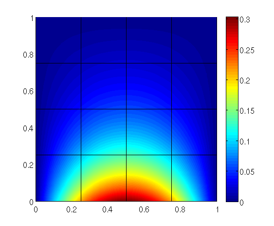
Finally, the solution u is stored in 'inhomNeumann.mat' file using graphics.MatlabBinaryGraphics. To this end, the shape functions are computed on equidistant points using the trapezoidal quadrature rule.

86  hp2D.IntegrableQuad.setTensor(concepts.TRAPEZE, True, 8 )
87  space.recomputeShapefunctions()
88  graphics.MatlabBinaryGraphics(spc = space, filename = "inhomNeumann", sol = sol)

Results

Output of the program:

Mesh: Import2dMesh(ncell = 1)
RHS Vector:
Vector(132, [ 1.678744e-01, 0.000000e+00, 1.570060e-02, 5.980456e-03, 0.000000e+00, 0.000000e+00, 0.000000e+00, 0.000000e+00, 0.000000e+00, 0.000000e+00, 0.000000e+00, 0.000000e+00, 2.374103e-01, 0.000000e+00, 3.790460e-02, 2.477186e-03, 0.000000e+00, 0.000000e+00, 0.000000e+00, 0.000000e+00, 0.000000e+00, 0.000000e+00, 0.000000e+00, 0.000000e+00, 0.000000e+00, 0.000000e+00, 0.000000e+00, 0.000000e+00, 0.000000e+00, 0.000000e+00, 0.000000e+00, 0.000000e+00, 0.000000e+00, 0.000000e+00, 0.000000e+00, 0.000000e+00, 0.000000e+00, 0.000000e+00, 0.000000e+00, 0.000000e+00, 0.000000e+00, 0.000000e+00, 1.678744e-01, 0.000000e+00, 3.790460e-02, -2.477186e-03, 0.000000e+00, 0.000000e+00, 0.000000e+00, 0.000000e+00, 0.000000e+00, 0.000000e+00, 0.000000e+00, 0.000000e+00, 1.570060e-02, -5.980456e-03, 0.000000e+00, 0.000000e+00, 0.000000e+00, 0.000000e+00, 0.000000e+00, 0.000000e+00, 0.000000e+00, 0.000000e+00, 0.000000e+00, 0.000000e+00, 0.000000e+00, 0.000000e+00, 0.000000e+00, 0.000000e+00, 0.000000e+00, 0.000000e+00, 0.000000e+00, 0.000000e+00, 0.000000e+00, 0.000000e+00, 0.000000e+00, 0.000000e+00, 0.000000e+00, 0.000000e+00, 0.000000e+00, 0.000000e+00, 0.000000e+00, 0.000000e+00, 0.000000e+00, 0.000000e+00, 0.000000e+00, 0.000000e+00, 0.000000e+00, 0.000000e+00, 0.000000e+00, 0.000000e+00, 0.000000e+00, 0.000000e+00, 0.000000e+00, 0.000000e+00, 0.000000e+00, 0.000000e+00, 0.000000e+00, 0.000000e+00, 0.000000e+00, 0.000000e+00, 0.000000e+00, 0.000000e+00, 0.000000e+00, 0.000000e+00, 0.000000e+00, 0.000000e+00, 0.000000e+00, 0.000000e+00, 0.000000e+00, 0.000000e+00, 0.000000e+00, 0.000000e+00, 0.000000e+00, 0.000000e+00, 0.000000e+00, 0.000000e+00, 0.000000e+00, 0.000000e+00, 0.000000e+00, 0.000000e+00, 0.000000e+00, 0.000000e+00, 0.000000e+00, 0.000000e+00, 0.000000e+00, 0.000000e+00, 0.000000e+00, 0.000000e+00, 0.000000e+00, 0.000000e+00])
System Matrix:
SparseMatrix(132x132, HashedSparseMatrix: 1794 (10.2961%) entries bound.)
Solver:
Mumps(n = 132)
Solution:
Vector(132, [ 2.138851e-01, 9.326650e-02, 3.516756e-02, 5.583589e-03, -4.883840e-02, 3.355068e-03, 1.532811e-02, 2.432564e-03, -8.058410e-03, 5.673075e-04, -1.285410e-03, 9.597194e-05, 3.024792e-01, 1.318988e-01, 8.490199e-02, 2.312798e-03, -6.906793e-02, 4.744783e-03, 3.700534e-02, -1.007601e-03, -1.945472e-02, 1.369602e-03, -5.324341e-04, 3.975288e-05, 5.610624e-02, 3.967310e-02, -2.989946e-02, 2.111419e-03, 1.574144e-02, 4.286670e-04, -2.114211e-02, -1.492999e-03, -8.387079e-03, 5.915169e-04, -2.281498e-04, 1.597013e-05, 6.520320e-03, 1.034894e-03, -3.474042e-03, 2.450143e-04, -5.508022e-04, 3.855529e-05, 2.138851e-01, 9.326650e-02, 8.490199e-02, -2.312798e-03, -4.883840e-02, 3.355068e-03, 3.700534e-02, -1.007601e-03, -1.945472e-02, 1.369602e-03, 5.324341e-04, -3.975288e-05, 3.516756e-02, -5.583589e-03, 1.532811e-02, 2.432564e-03, -8.058410e-03, 5.673075e-04, 1.285410e-03, -9.597194e-05, 3.967310e-02, 6.520320e-03, 1.034894e-03, -2.114211e-02, -1.492999e-03, -3.474042e-03, 2.450143e-04, 5.508022e-04, -3.855529e-05, 1.574144e-02, 4.286670e-04, -8.387079e-03, 5.915169e-04, 2.281498e-04, -1.597013e-05, 1.459270e-02, 2.063719e-02, -8.630098e-03, 6.986304e-04, 5.790065e-03, -1.576721e-04, -1.220480e-02, -9.880126e-04, -3.424278e-03, 2.772246e-04, 9.325616e-05, -7.553547e-06, 2.398323e-03, 3.806541e-04, -1.418383e-03, 1.148302e-04, 2.251403e-04, -1.823587e-05, -2.320734e-03, -4.064907e-04, -3.814143e-04, 6.680687e-05, 6.053633e-05, -1.060309e-05, -3.282014e-03, -5.748646e-04, -9.208157e-04, 1.612860e-04, 2.507497e-05, -4.391942e-06, 1.459270e-02, -8.630098e-03, 6.986304e-04, 2.398323e-03, 3.806541e-04, -1.418383e-03, 1.148302e-04, -2.251403e-04, 1.823587e-05, 5.790065e-03, -1.576721e-04, -3.424278e-03, 2.772246e-04, -9.325616e-05, 7.553547e-06, -2.320734e-03, -4.064907e-04, -9.208157e-04, 1.612860e-04, -2.507497e-05, 4.391942e-06, -3.814143e-04, 6.680687e-05, -6.053633e-05, 1.060309e-05])

Matlab plot of the solution: Matlab output

Complete Source Code

1 # import modules from package
2 from libconceptspy import concepts
3 from libconceptspy import graphics
4 from libconceptspy import hp1D
5 from libconceptspy import hp2D
6 
7 import os
8 from sys import exit
9 from mpi4py import MPI
10 
11 SOURCEDIR = os.environ['CONCEPTSPATH']
12 
13 def main():
14  try:
15  mesh = concepts.Import2dMesh(coord = SOURCEDIR + "/applications/unitsquareCoordinates.dat",
16  elms = SOURCEDIR + "/applications/unitsquareElements.dat",
17  boundary = SOURCEDIR + "/applications/unitsquareEdges.dat"
18  )
19  print ('Mesh:')
20  print (mesh)
21  except RuntimeError:
22  print("Mesh import error")
23  else:
24  graphics.MeshEPS_r(msh = mesh, filename = "mesh.eps", scale=100, greyscale=1.0, nPoints=1)
25 
26  boundaryConditions = concepts.BoundaryConditions()
27  for i in range(2,5):
28  boundaryConditions.add(attrib = i, bcObject = concepts.Boundary(type = concepts.Boundary.DIRICHLET))
29 
30 
31  NeumannFormula = concepts.ParsedFormula_r(formula = "(sin(pi*x))")
32  attrNeumann = concepts.Set_uint(1)
33 
34 
35  levelOfRefinement = 2
36  polynomialDegree = 3
37  space = hp2D.hpAdaptiveSpaceH1(msh = mesh, l = levelOfRefinement,
38  p = polynomialDegree, bc = boundaryConditions)
39  space.rebuild()
40  graphics.MeshEPS_r(spc = space, filename = "space.eps", scale=100, greyscale=1.0, nPoints=1)
41 
42 
43  tscpNeumann = hp2D.TraceSpace(spc = space, edgeAttr = attrNeumann)
44 
45 
46  lformNeumann = hp1D.Riesz_r(frm = NeumannFormula)
47  rhs = concepts.Vector_r(spc = tscpNeumann, lf = lformNeumann)
48  print('\nRHS Vector:')
49  print(rhs)
50 
51 
52  la = hp2D.Laplace_r()
53  A = concepts.SparseMatrix_r(spc = space, bf = la)
54  A.compress()
55 
56  id = hp2D.Identity_r()
57  M = concepts.SparseMatrix_r(spc = space, bf = id)
58  M.compress()
59  M.addInto(A,1.0)
60  print('\nSystem Matrix:')
61  print(A)
62 
63 
64  solver = concepts.Mumps_r(A = A)
65  sol = concepts.Vector_r(spc = space)
66  solver(fncY = rhs, fncX = sol)
67  print('\nSolver:')
68  print(solver)
69  print('\nSolution:')
70  print(sol)
71 
72 
73  hp2D.IntegrableQuad.setTensor(concepts.TRAPEZE, True, 8 )
74  space.recomputeShapefunctions()
75  graphics.MatlabBinaryGraphics(spc = space, filename = "inhomNeumann", sol = sol)
76 
77 if __name__ == "__main__":
78  main()
Builds the trace space of an FE space.
Definition: traces.hh:52
Class that allows to store graphical infomations in .mat files to use them in Matlab.
Class to describe an element of the boundary.
Definition: boundary.hh:35
Page URL: http://wiki.math.ethz.ch/bin/view/Concepts/WebHome
21 August 2020
© 2020 Eidgenössische Technische Hochschule Zürich