In this tutorial the implementation of inhomogeneous Dirichlet boundary conditions using Lagrangian multipliers is shown.
The mesh is read from three files containing the coordinates, the elements and the boundary attributes of the mesh.
In our example, the edges are given the following attributes: 1 (bottom), 2 (right), 3 (top) and 4 (left).
If there is an error reading those files, then an exception error message is returned.
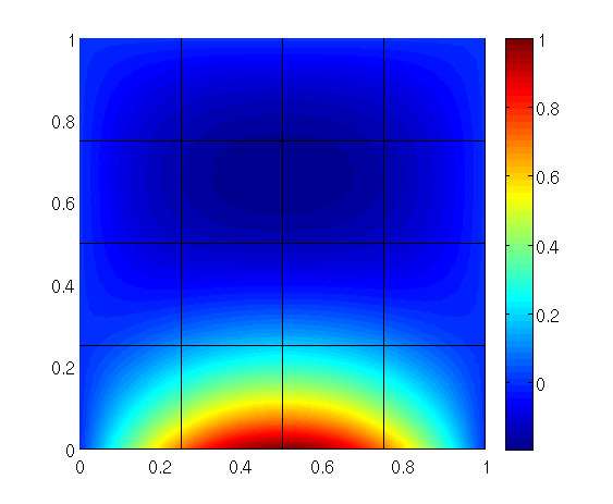
else, the mesh is plotted using scaling factor of 100, a greyscale of 1.0 and one point per edge.
The space is built using the mesh, a refinement factor of 2 and a polynomial degree to 3. Then the elements of the space are built and the space is plotted.
The right hand side is computed. First we calculate the vector corresponding to the linear form of the source term
then the vector that corresponds to the inhomogeneous Dirichlet boundary condition is built
and finally, these two vectors are put together in a block vector.
The system matrix is also assembled as a block matrix. First we account for the bilinear forms hp2D.Laplace_r and hp2D.Identity_r that build the upper right block.
We solve the equation using a Mumps solver.
Mesh: Import2dMesh(ncell = 1)
Space:
Trace Space:
TraceSpace(QuadEdgeFirst(EdgeNormalVectorRule()), dim = 169, nelm = 16)
Dual Space:
DualSpace(dim = 48, nelm = 16)
RHS Vector 2D:
Vector(169, [-5.494815e-02, -1.219900e-01, -2.708292e-01, -1.219900e-01, -1.893229e-02, -7.072544e-04, -4.203145e-02, -1.570171e-03, -4.203145e-02, -1.570171e-03, -1.893229e-02, -7.072544e-04, -6.523089e-03, -2.436833e-04, -2.436833e-04, -9.103287e-06, -1.296912e-01, -2.879265e-01, -2.143641e-02, -2.669927e-04, -4.468487e-02, -1.669295e-03, -4.759082e-02, 5.927486e-04, -7.385877e-03, -2.759145e-04, -9.199187e-05, -3.436544e-06, -3.061031e-01, -2.879265e-01, -5.059520e-02, -6.301685e-04, -5.059520e-02, -6.301685e-04, -4.759082e-02, 5.927486e-04, -8.362783e-03, -1.041593e-04, -1.041593e-04, -1.297316e-06, -1.296912e-01, -4.468487e-02, -1.669295e-03, -2.143641e-02, -2.669927e-04, -7.385877e-03, -9.199187e-05, -2.759145e-04, -3.436544e-06, -1.219900e-01, -2.708292e-01, -2.143641e-02, 2.669927e-04, -4.203145e-02, -1.570171e-03, -4.759082e-02, 5.927486e-04, -7.385877e-03, -2.759145e-04, 9.199187e-05, 3.436544e-06, -5.494815e-02, -1.219900e-01, -1.893229e-02, 7.072544e-04, -1.893229e-02, -7.072544e-04, -4.203145e-02, -1.570171e-03, -6.523089e-03, -2.436833e-04, 2.436833e-04, 9.103287e-06, -1.296912e-01, -2.879265e-01, -2.143641e-02, -2.669927e-04, -4.468487e-02, -1.669295e-03, -4.759082e-02, 5.927486e-04, -7.385877e-03, -9.199187e-05, 2.759145e-04, 3.436544e-06, -5.059520e-02, -6.301685e-04, -8.362783e-03, -1.041593e-04, 1.041593e-04, 1.297316e-06, -2.708292e-01, -2.879265e-01, -4.759082e-02, 5.927486e-04, -4.759082e-02, 5.927486e-04, -5.059520e-02, -6.301685e-04, -8.362783e-03, 1.041593e-04, 1.041593e-04, -1.297316e-06, -1.219900e-01, -2.143641e-02, 2.669927e-04, -4.203145e-02, -1.570171e-03, -7.385877e-03, 9.199187e-05, 2.759145e-04, -3.436544e-06, -5.494815e-02, -1.219900e-01, -1.893229e-02, 7.072544e-04, -1.893229e-02, -7.072544e-04, -4.203145e-02, -1.570171e-03, -6.523089e-03, 2.436833e-04, 2.436833e-04, -9.103287e-06, -1.296912e-01, -2.143641e-02, -2.669927e-04, -4.468487e-02, -1.669295e-03, -7.385877e-03, 2.759145e-04, 9.199187e-05, -3.436544e-06, -2.708292e-01, -1.219900e-01, -4.759082e-02, 5.927486e-04, -4.203145e-02, -1.570171e-03, -2.143641e-02, 2.669927e-04, -7.385877e-03, 9.199187e-05, -2.759145e-04, 3.436544e-06, -4.759082e-02, 5.927486e-04, -8.362783e-03, 1.041593e-04, -1.041593e-04, 1.297316e-06, -1.219900e-01, -2.143641e-02, 2.669927e-04, -4.203145e-02, -1.570171e-03, -7.385877e-03, 2.759145e-04, -9.199187e-05, 3.436544e-06, -5.494815e-02, -1.893229e-02, 7.072544e-04, -1.893229e-02, 7.072544e-04, -6.523089e-03, 2.436833e-04, -2.436833e-04, 9.103287e-06])
RHS Vector 1D:
Vector(48, [ 1.960099e-03, 0.000000e+00, 0.000000e+00, 0.000000e+00, 1.853134e-01, -9.727886e-04, -1.320752e-04, 2.620727e-01, -2.348519e-03, -5.470734e-05, 0.000000e+00, 0.000000e+00, 0.000000e+00, 1.853134e-01, -2.348519e-03, 5.470734e-05, 1.960099e-03, 2.864357e-17, -7.696566e-20, 4.296913e-22, -9.727886e-04, 1.320752e-04, 2.192284e-17, -6.524834e-20, 1.223657e-21, 1.186456e-17, -4.359754e-20, 1.831332e-21, 1.506967e-19, 1.134717e-17, -5.956612e-20, -8.087273e-21, -1.530942e-20, 2.160204e-21, 1.604733e-17, -1.438053e-19, -3.349858e-21, 0.000000e+00, 0.000000e+00, 0.000000e+00, 1.134717e-17, -1.438053e-19, 3.349858e-21, 1.200215e-19, 0.000000e+00, 0.000000e+00, -5.956612e-20, 8.087273e-21])
RHS Vector:
Vector(217, [-5.494815e-02, -1.219900e-01, -2.708292e-01, -1.219900e-01, -1.893229e-02, -7.072544e-04, -4.203145e-02, -1.570171e-03, -4.203145e-02, -1.570171e-03, -1.893229e-02, -7.072544e-04, -6.523089e-03, -2.436833e-04, -2.436833e-04, -9.103287e-06, -1.296912e-01, -2.879265e-01, -2.143641e-02, -2.669927e-04, -4.468487e-02, -1.669295e-03, -4.759082e-02, 5.927486e-04, -7.385877e-03, -2.759145e-04, -9.199187e-05, -3.436544e-06, -3.061031e-01, -2.879265e-01, -5.059520e-02, -6.301685e-04, -5.059520e-02, -6.301685e-04, -4.759082e-02, 5.927486e-04, -8.362783e-03, -1.041593e-04, -1.041593e-04, -1.297316e-06, -1.296912e-01, -4.468487e-02, -1.669295e-03, -2.143641e-02, -2.669927e-04, -7.385877e-03, -9.199187e-05, -2.759145e-04, -3.436544e-06, -1.219900e-01, -2.708292e-01, -2.143641e-02, 2.669927e-04, -4.203145e-02, -1.570171e-03, -4.759082e-02, 5.927486e-04, -7.385877e-03, -2.759145e-04, 9.199187e-05, 3.436544e-06, -5.494815e-02, -1.219900e-01, -1.893229e-02, 7.072544e-04, -1.893229e-02, -7.072544e-04, -4.203145e-02, -1.570171e-03, -6.523089e-03, -2.436833e-04, 2.436833e-04, 9.103287e-06, -1.296912e-01, -2.879265e-01, -2.143641e-02, -2.669927e-04, -4.468487e-02, -1.669295e-03, -4.759082e-02, 5.927486e-04, -7.385877e-03, -9.199187e-05, 2.759145e-04, 3.436544e-06, -5.059520e-02, -6.301685e-04, -8.362783e-03, -1.041593e-04, 1.041593e-04, 1.297316e-06, -2.708292e-01, -2.879265e-01, -4.759082e-02, 5.927486e-04, -4.759082e-02, 5.927486e-04, -5.059520e-02, -6.301685e-04, -8.362783e-03, 1.041593e-04, 1.041593e-04, -1.297316e-06, -1.219900e-01, -2.143641e-02, 2.669927e-04, -4.203145e-02, -1.570171e-03, -7.385877e-03, 9.199187e-05, 2.759145e-04, -3.436544e-06, -5.494815e-02, -1.219900e-01, -1.893229e-02, 7.072544e-04, -1.893229e-02, -7.072544e-04, -4.203145e-02, -1.570171e-03, -6.523089e-03, 2.436833e-04, 2.436833e-04, -9.103287e-06, -1.296912e-01, -2.143641e-02, -2.669927e-04, -4.468487e-02, -1.669295e-03, -7.385877e-03, 2.759145e-04, 9.199187e-05, -3.436544e-06, -2.708292e-01, -1.219900e-01, -4.759082e-02, 5.927486e-04, -4.203145e-02, -1.570171e-03, -2.143641e-02, 2.669927e-04, -7.385877e-03, 9.199187e-05, -2.759145e-04, 3.436544e-06, -4.759082e-02, 5.927486e-04, -8.362783e-03, 1.041593e-04, -1.041593e-04, 1.297316e-06, -1.219900e-01, -2.143641e-02, 2.669927e-04, -4.203145e-02, -1.570171e-03, -7.385877e-03, 2.759145e-04, -9.199187e-05, 3.436544e-06, -5.494815e-02, -1.893229e-02, 7.072544e-04, -1.893229e-02, 7.072544e-04, -6.523089e-03, 2.436833e-04, -2.436833e-04, 9.103287e-06, 1.960099e-03, 0.000000e+00, 0.000000e+00, 0.000000e+00, 1.853134e-01, -9.727886e-04, -1.320752e-04, 2.620727e-01, -2.348519e-03, -5.470734e-05, 0.000000e+00, 0.000000e+00, 0.000000e+00, 1.853134e-01, -2.348519e-03, 5.470734e-05, 1.960099e-03, 2.864357e-17, -7.696566e-20, 4.296913e-22, -9.727886e-04, 1.320752e-04, 2.192284e-17, -6.524834e-20, 1.223657e-21, 1.186456e-17, -4.359754e-20, 1.831332e-21, 1.506967e-19, 1.134717e-17, -5.956612e-20, -8.087273e-21, -1.530942e-20, 2.160204e-21, 1.604733e-17, -1.438053e-19, -3.349858e-21, 0.000000e+00, 0.000000e+00, 0.000000e+00, 1.134717e-17, -1.438053e-19, 3.349858e-21, 1.200215e-19, 0.000000e+00, 0.000000e+00, -5.956612e-20, 8.087273e-21])
System Matrix A11:
SparseMatrix(169x169, HashedSparseMatrix: 1785 (6.24978%) entries bound.)
System Matrix M11:
SparseMatrix(169x169, HashedSparseMatrix: 2809 (9.83509%) entries bound.)
System Matrix M12:
SparseMatrix(169x169, HashedSparseMatrix: 2809 (9.83509%) entries bound.)
System Matrix M21:
SparseMatrix(48x169, HashedSparseMatrix: 112 (1.38067%) entries bound.)
System Matrix A:
SparseMatrix(217x217, HashedSparseMatrix: 3033 (6.44099%) entries bound.)
Solver:
Mumps(n = 217)
Solution u:
Vector(169, [-3.843730e-05, 7.069574e-01, 1.145216e-01, 2.745231e-17, 1.167346e-01, 1.849053e-02, -2.470302e-01, 1.513115e-02, -3.521483e-02, 1.222784e-02, -1.767987e-16, -1.300331e-16, -1.010858e-01, 1.657205e-02, 9.822506e-03, -6.715120e-03, 9.997888e-01, 1.865335e-01, 2.818223e-01, 7.659027e-03, -3.290883e-01, 1.852945e-02, 6.508946e-02, -4.285731e-03, -8.302083e-02, 4.354588e-03, -1.070311e-03, 3.682207e-04, -1.390846e-01, -1.183699e-01, -1.754996e-01, 7.990479e-03, -2.459961e-02, 2.422382e-03, -1.271322e-01, -5.897441e-03, -4.730355e-02, 2.067389e-03, -6.100085e-04, -3.252949e-05, 8.392560e-18, -7.963128e-02, 6.484164e-03, -6.632734e-17, -6.022298e-17, -2.783892e-02, 1.551738e-03, -3.120827e-03, 2.829607e-04, 7.069574e-01, 1.145216e-01, 2.818223e-01, -7.659027e-03, -2.470302e-01, 1.513115e-02, 6.508946e-02, -4.285731e-03, -8.302083e-02, 4.354588e-03, 1.070311e-03, -3.682207e-04, -3.843730e-05, 1.337389e-16, 1.167346e-01, -1.849053e-02, -2.204895e-17, -2.867429e-17, -3.521483e-02, 1.222784e-02, -1.010858e-01, 1.657205e-02, -9.822506e-03, 6.715120e-03, 9.411970e-17, -1.183699e-01, -1.148842e-16, 7.434135e-17, -7.963128e-02, 6.484164e-03, -1.271322e-01, -5.897441e-03, -2.783892e-02, 1.551738e-03, 3.120827e-03, -2.829607e-04, -2.459961e-02, 2.422382e-03, -4.730355e-02, 2.067389e-03, 6.100085e-04, 3.252949e-05, -1.455747e-01, -1.813021e-01, -8.576168e-02, 1.351167e-03, -3.808912e-02, -1.479664e-03, -1.169903e-01, -2.261285e-03, -3.094120e-02, 7.818221e-04, 1.733609e-04, -1.052648e-04, 5.297275e-17, 4.508856e-17, -3.546363e-17, -7.793839e-02, 5.447318e-03, -2.107821e-02, -3.758636e-04, 2.052405e-03, 1.006130e-04, -3.516085e-17, 4.849705e-17, -6.076754e-18, -6.568048e-18, -9.181996e-18, 5.938771e-18, -9.353945e-02, 2.845041e-03, -7.477510e-02, -1.400772e-02, -1.402845e-02, -7.228221e-03, 6.720056e-17, -1.363958e-19, 1.186490e-17, -1.120372e-01, 1.162147e-03, -1.943362e-02, 1.840870e-03, -6.726377e-04, 1.466294e-04, -1.455747e-01, -7.018279e-18, -8.576168e-02, 1.351167e-03, -7.793839e-02, 5.447318e-03, 7.994743e-17, -2.645529e-18, -2.107821e-02, -3.758636e-04, -2.052405e-03, -1.006130e-04, -3.808912e-02, -1.479664e-03, -3.094120e-02, 7.818221e-04, -1.733609e-04, 1.052648e-04, 4.682683e-17, -1.640647e-17, 1.921618e-17, -9.353945e-02, 2.845041e-03, -1.943362e-02, 1.840870e-03, 6.726377e-04, -1.466294e-04, 3.588635e-17, 2.192255e-18, -4.324464e-18, 2.505082e-17, -1.383750e-17, -7.477510e-02, -1.400772e-02, 1.402845e-02, 7.228221e-03])
Lagrangian lambda:
Vector(48, [-2.599760e-01, -3.564760e-01, 5.334279e+00, -3.591746e+00, 3.312759e+00, -2.286376e+00, 8.518971e+00, 4.523683e+00, -2.194781e+00, 2.776326e+00, 7.677355e-01, -1.142425e+00, 2.714910e+00, 3.312759e+00, -2.194781e+00, -2.776326e+00, -2.599760e-01, -3.564760e-01, 5.334279e+00, -3.591746e+00, -2.286376e+00, -8.518971e+00, 7.677355e-01, -1.142425e+00, 2.714910e+00, 8.660466e-01, -7.911928e-01, 2.372638e-01, 4.703880e-01, 9.287585e-01, 2.710241e-01, 5.898491e-01, 1.557665e-01, -4.119058e-01, 1.152213e+00, -4.279965e-01, 5.506984e-01, 8.660466e-01, -7.911928e-01, 2.372638e-01, 9.287585e-01, -4.279965e-01, -5.506984e-01, 4.703880e-01, 1.557665e-01, -4.119058e-01, 2.710241e-01, -5.898491e-01])
![\[ - \Delta u + u = f \]](form_719.png)
 with source term
 ![\[ f(x,y) = -5\exp\left(-(x-1/2)^2-(y-1/2)^2\right) \]](form_720.png)
 on the boundary
  of
of  where
where ![\[ g = \begin{cases} \sin \pi x, &(x,y)\in\Gamma_{\rm inh}=\{(x,y)\in\partial\Omega\mid y=0\},\\ 0, &(x,y)\in\partial\Omega\setminus\Gamma_{\rm inh}. \end{cases} \]](form_730.png)
 that satisfies the boundary conditions and
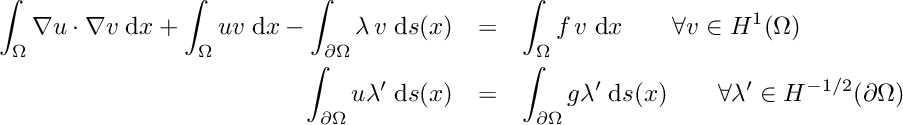
 ![\[ \int_{\Omega}\nabla u\cdot\nabla v\;{\rm d}x + \int_{\Omega} u\,v\;{\rm d}x - \int_{\partial\Omega} \partial_n u \,v \;{\rm d}s(x) = \int_{\Omega} f\,v\;{\rm d}x, \]](form_732.png)
 . In order to incorporate the boundary conditions into the variational formulation, we introduce the Lagrangian multiplier
  defined by
  . The space
  of the Lagrangian multiplier is the dual space of the trace space
  of
of  on the boundary
  such that