parallelizationTutorial.cc
On this page you find the easy example of an elliptic partial differential equation that was already discussed in How to get started.However, in this tutorial the PDE is solved in parallel.
Introduction
Recall that the model problem is to find a finite element approximation to the unique solution  of the following elliptic PDE with homogeneous Dirichlet boundary conditions
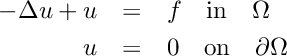
with the right hand side  and
and  . The discrete variational formulation of this PDE reads: find
  such that
![\[ \int_{\Omega} \nabla u_h \cdot \nabla v_h \, {\rm d}\mathbf{x} + \int_\Omega u_h v_h \, {\rm d}\mathbf{x} = \int_\Omega f v_h {\rm d}\mathbf{x} \qquad \forall v_h \in V_h. \]](form_124.png)
Differences to the sequential version
If you are familiar with the sequential version, there are only some minors changes to apply.
Use MPI
The program should start with
@code
MPI_Init(&argc, &argv);
@endcode
and end with
@code
MPI_Finalize();
@endcode
In addition, we have to retrieve the number of processes using the command MPI_Comm_size and the current process using the command MPI_Comm_rank. By convention, the master process is the process of rank 0.
@code
int nbParts; MPI_Comm_size(MPI_COMM_WORLD, &nbParts);
int part; MPI_Comm_rank(MPI_COMM_WORLD, &part);
bool master = (part == 0);
@endcode
Graph partitioning
The graph partitioning is done with the generic concepts::SpaceGraph class.
@code
#include "space.hh"
concepts::SpaceGraph<hp2D::hpAdaptiveSpaceH1> sgraph(space);
sgraph.SplitGraph(nbParts);
@endcode
Matrix assembling
For the matrix assembling, we have to use the getSubDomain method as an additional parameter.
For example, we replace the build of the stiffness matrix  and mass matrix
@code
concepts::SparseMatrix<Real> S(space, la);
concepts::SparseMatrix<Real> M(space, id);
@endcode
by the following builds
@code
concepts::SparseMatrix<Real> S(space, la, sgraph.getSubDomain(part));
concepts::SparseMatrix<Real> M(space, id, sgraph.getSubDomain(part));
@endcode
Solving process
The solving process does not differ very much from what is done in the sequential version. However, we have to use the concepts::MumpsOverlap class for solving.
We declare for each process the solver
@code
concepts::MumpsOverlap<Real>* solver = new concepts::MumpsOverlap<Real>(S, part);
@endcode
and we differentiate two cases:
- If the process is the master process, we build the right hand side, solve and do the post-processing of the solution as usual.
- If, on the other hand, the process is not the master process, we simply call the solver.
The associated code is
@code
if (master)
{
... Treatment before calling solver
(*solver)(rhs, sol);
... Treatment after calling solver
}
else
{
(*solver)();
}
@endcode
Commented Program
Now let us see how to parallelly calculate the FEM-approximation to the solution of the PDE with Concepts. First we have to include some headers to use the functions of specific Concepts packages.
The package hp2D includes all functions that are needed to build a representation of the hp-finite element space in two dimensions. The package operator.hh includes the data structures for Concepts matrices and linear solvers, the package formula allows you to represent the right hand side via its symbolic formula and the package graphics is used for the graphical output of the mesh and the solution.
The instruction
allows us to use the datatype concepts::Real just by typing Real .
Next we start with the actual code, consisting of a main program.
Since we use MPI, we also have to initialize the MPI process using the instruction MPI_Init .
First, we load the geometry that contains several cells.
Now we prescribe homogeneous Dirichlet boundary conditions to all edges of attributes  to
to  , i.e. to all edges.
With the mesh and the boundary conditions at hand we can build the hp-finite element space.
This is a finite element space on the square, with a twice refined mesh (a single refinement of a two dimensional mesh divides an element in the mesh into four elements, so in our case we have 16 subelements in our square) and polynomial degree six on every element.
Now we split the graph associated to this mesh into  parts, where is the number of MPI process given by the command
 mpirun -np N
and we build the matrices S (the stiffness matrix, corresponding to the  term) and
 M (the mass matrix, corresponding to the  term)
term)
Next point is that we build the solver (more precisely: the subpart of the solver corresponding to each thread)
The treatment of the right hand side and the way we call the solver now depend on whether or not we are on the master thread.
On the master thread, we build the right hand side and we call the solver.
On all other threads, we simply call the solver.
Now we want to compute the error between the computed and the exact solution of PDE. Also this task can be done in parallel. Next we distribute the solution vector to all other threads.
The formulas of computed and exact solution are build by
Next we compute the  on each subdomain.
Finally we collect the values from all threads