Introduction
Two dimensional FEM in Concepts. This code features high order Ansatz functions and irregular meshes (local, anisotropic refinements in h and p). All classes for the hp-FEM in two dimensions can be found in the namespace hp2D.
The equation solved is a reaction-diffusion equation (without reaction term)
![\[ - \Delta u = 0 \]](form_151.png)
on the L shaped domain (-1,1)2 \ (0,1)x(-1,0) with mixed boundary conditions chosen such that the exact solution is  . The linear system is solved using CG or a direct solver.
 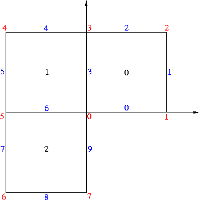 The boundary conditions are homogeneous Dirichlet on the edges 0 and 9 and non-zero Neumann on the rest of the boundary.
The exact solution is .
The relative error in energy norm is computed.
Contents
- Commented Program
- Results
- Complete Source Code
Commented Program
System include files.
Concepts include files. hp2D.hh is for the high order method.
#include "formula.hh"
#include "function.hh"
#include "graphics.hh"
#include "operator.hh"
#include "space.hh"
With this using directive, we do not need to prepend concepts:: before Real everytime.
Main Program
The mesh is read from three file containing the coordinates, the elements and the boundary conditions of the mesh.
int main(int argc, char** argv) {
try {
SOURCEDIR "/applications/lshape2DElements.dat",
SOURCEDIR "/applications/lshape2DBoundary.dat");
std::cout << "msh = " << msh << std::endl;
The boundary conditions are different for each segment of the boundary.
Using the mesh and the boundary conditions, the space can be built. Note that the elements are not yet created as this is an adaptive space. It builds its elements only on request via hp2D::Space::rebuild().
Now, the loop over the different computational levels is initialized.
Now, it is time to build the elements of the space. The newly built space is printed.
The right hand side is computed. In our case, the vector rhs only contains the integrals of the Neumann boundary conditions as the right hand side f is 0.
The stiffness matrix is computed from the bilinear form hp2D::Laplace.
The next part is the linear solver. We use a diagonally preconditioned conjugate gradient solver.
Now, everything is prepared to solve the linear system.
sol is an empty vector to hold the solution of the linear system.
Some immediate statistics of the solver.
The energy of the FE solution in sol can be computed by multiplying sol and rhs. It is compared to the exact energy.
If there are further computations (ie. i < 2), the space is refined using hp2D::APrioriRefinement towards the vertex carying the singularity (the origin). This information has to be given a-priori by the user.
Finally, exceptions are caught and a sane return value is given back.
Results
Output of the program:
msh = Import2dMesh(ncell = 3)
BoundaryConditions(1: Boundary(DIRICHLET, (0)), 2: Boundary(NEUMANN, ParsedFormula( (1/(1+y*y)^(2/3)) * (sin(2/3*atan(y)) - y*cos(2/3*atan(y)))*2/3 )), 3: Boundary(NEUMANN, ParsedFormula( 2/3/((1+x*x)^(2/3)) * (sin(2/3*atan(1/x)) + x*cos(2/3*atan(1/x))) )), 4: Boundary(NEUMANN, ParsedFormula( 2/3/((1+x*x)^(2/3)) * (sin(2/3*(atan(1/x)+
pi)) + x*cos(2/3*(atan(1/x)+
pi))) )), 5: Boundary(NEUMANN, ParsedFormula( 2/3/((1+y*y)^(2/3)) * (sin(2/3*(atan(-y)+
pi)) + y*cos(2/3*(atan(-y)+
pi))) )), 6: Boundary(NEUMANN, ParsedFormula( 2/3/((1+y*y)^(2/3)) * (sin(2/3*(atan(-y)+
pi)) + y*cos(2/3*(atan(-y)+
pi))) )), 7: Boundary(NEUMANN, ParsedFormula( 2/3/((1+x*x)^(2/3)) * (sin(2/3*(atan(-1/x)+
pi)) - x*cos(2/3*(atan(-1/x)+
pi))) )), 8: Boundary(DIRICHLET, (0)), 0: Boundary(FREE, (0)))
--
i = 0
space = Space(dim = 5, nelm = 3)
matrix: SparseMatrix(5x5, HashedSparseMatrix: 15 (60%) entries bound.)
solver = CG(solves SparseMatrix(5x5, HashedSparseMatrix: 15 (60%) entries bound.), eps = 9.73773e-33, it = 2, relres = 0)
FE energy = 1.7449, rel. energy error = 0.0497347
i = 1
space = Space(dim = 16, nelm = 12)
matrix: SparseMatrix(16x16, HashedSparseMatrix: 90 (35.1562%) entries bound.)
solver = CG(solves SparseMatrix(16x16, HashedSparseMatrix: 90 (35.1562%) entries bound.), eps = 1.66559e-33, it = 6, relres = 0)
FE energy = 1.79339, rel. energy error = 0.0233299
i = 2
space = Space(dim = 50, nelm = 21)
matrix: SparseMatrix(50x50, HashedSparseMatrix: 402 (16.08%) entries bound.)
solver = CG(solves SparseMatrix(50x50, HashedSparseMatrix: 402 (16.08%) entries bound.), eps = 6.74911e-13, it = 17, relres = 0)
FE energy = 1.81761, rel. energy error = 0.0101395
Complete Source Code
- Author
- Philipp Frauenfelder, 2004
#include <iostream>
#include "formula.hh"
#include "function.hh"
#include "graphics.hh"
#include "operator.hh"
#include "space.hh"
int main(int argc, char** argv) {
try {
SOURCEDIR "/applications/lshape2DElements.dat",
SOURCEDIR "/applications/lshape2DBoundary.dat");
std::cout << "msh = " << msh << std::endl;
("( (1/(1+y*y)^(2/3)) * (sin(2/3*atan(y)) - y*cos(2/3*atan(y)))*2/3 )")));
("( 2/3/((1+x*x)^(2/3)) * (sin(2/3*atan(1/x)) + x*cos(2/3*atan(1/x))) )")));
("( 2/3/((1+x*x)^(2/3)) * (sin(2/3*(atan(1/x)+pi)) + x*cos(2/3*(atan(1/x)+pi))) )")));
("( 2/3/((1+y*y)^(2/3)) * (sin(2/3*(atan(-y)+pi)) + y*cos(2/3*(atan(-y)+pi))) )")));
("( 2/3/((1+y*y)^(2/3)) * (sin(2/3*(atan(-y)+pi)) + y*cos(2/3*(atan(-y)+pi))) )")));
("( 2/3/((1+x*x)^(2/3)) * (sin(2/3*(atan(-1/x)+pi)) - x*cos(2/3*(atan(-1/x)+pi))) )")));
std::cout << bc << std::endl;
std::cout << "--" << std::endl;
for (uint i = 0; i < 3; ++i) {
std::cout << "i = " << i << std::endl;
std::cout << " space = " << space << std::endl;
std::cout << " matrix: " << stiff << std::endl;
solver(rhs, sol);
std::cout << " solver = " << solver << std::endl;
const Real exenergy = 1.8362264461350097;
const Real FEenergy = sol*rhs;
const Real relError = fabs(FEenergy - exenergy)/exenergy;
std::cout << " FE energy = " << FEenergy
<< ", rel. energy error = " << relError << std::endl;
if (i < 2) {
int pMax[2] = { 1, 1 };
post(refineSpace);
}
}
}
std::cout << e << std::endl;
return 1;
}
return 0;
}