On this page you find an easy example of an elliptic partial differential equation (PDE) solved with Concepts. Starting with this PDE, we derive its associated variational formulation and solve it numerically. This example is the standard setting in the Concepts tutorials where you can find many extensions to this simple code.

Introduction

We want to solve the following elliptic PDE with homogeneous Dirichlet boundary conditions

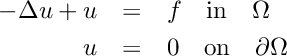
$\begin{eqnarray*} - \Delta u + u &=& f \quad \textrm{in} \quad \Omega\\ u &=& 0 \quad \textrm{on} \quad \partial \Omega\ \end{eqnarray*}$

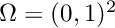with the right hand side $f(x,y) = (2 \pi^2 +1)\sin(\pi x) \sin(\pi y)$ and $\Omega = (0,1)^2$ . This problem has the unique solution $u(x,y) = \sin(\pi x) \sin(\pi y)$ .

To solve this problem with Concepts, we first need its variational formulation. Let $H_0^1(\Omega)$ be the Sobolev space of square integrable and weak differentiable functions with vanishing trace on $\partial \Omega$ . Then we seek the weak solution $u \in H_0^1(\Omega)$ that satisfies

$- \int_{\Omega} \Delta u v \, {\rm d}\mathbf{x} + \int_\Omega u v \, {\rm d}\mathbf{x} = \int_\Omega f v \, {\rm d}\mathbf{x} \qquad \forall v \in H_0^1(\Omega).$

Using integration by parts (Gauss theorem), this is equivalent to

$\int_{\Omega} \nabla u \cdot \nabla v \, {\rm d}\mathbf{x} - \int_{\partial \Omega} \underline{n} \cdot \nabla u \, v \, {\rm d}s(\mathbf{x})+ \int_\Omega u v \, {\rm d}\mathbf{x} = \int_\Omega f v \, {\rm d}\mathbf{x} \qquad \forall v \in H_0^1(\Omega),$

where $\underline{n}$ denotes the unit normal vector outward to $\Omega$ . Using that $v \in H_0^1(\Omega)$ has vanishing trace, we get

$\int_{\Omega} \nabla u \cdot \nabla v \, {\rm d}\mathbf{x} + \int_\Omega u v \, {\rm d}\mathbf{x} = \int_\Omega f v \, {\rm d}\mathbf{x} \qquad \forall v \in H_0^1(\Omega).$

This is the variational formulation of our problem. Let now $V_h \subseteq H_0^1$ be a finite dimensional subspace of . The Galerkin approximation of our solution in the space is given as the (unique) solution $u_h \in V_h$ that fulfills the equation

$\int_{\Omega} \nabla u_h \cdot \nabla v_h \, {\rm d}\mathbf{x} + \int_\Omega u_h v_h \, {\rm d}\mathbf{x} = \int_\Omega f v_h {\rm d}\mathbf{x} \qquad \forall v_h \in V_h.$

Let $\phi_1, ..., \phi_N$ be a basis of the space , then we can find a unique vector $\alpha = (\alpha_i)_{i = 1,...,N}$ such that $\sum_i \alpha_i \phi_i = u_h$ . Plugging this into the equation above and using the linearity of the integral, we obtain the linear equation

$\sum_k \alpha_k \left( \int_\Omega \nabla \phi_k \cdot \nabla \phi_j \, {\rm d}\mathbf{x} + \int_\Omega \phi_k \phi_j \, {\rm d}\mathbf{x} \right) = \int_\Omega f \phi_j \, {\rm d}\mathbf{x} \qquad \forall j \in \{ 1, ..., N\}.$

For $s_{k,j}:= \int_\Omega \nabla \phi_k \nabla \phi_j \,{\rm d}\mathbf{x}$ , $m_{k,j}:= \int_\Omega \phi_k \phi_j \,{\rm d}\mathbf{x}$ and $b_{j}:= \int_\Omega f \phi_j \,{\rm d}\mathbf{x}$ and matrices $S = (s_{ij})_{i j}$ , $M = (m_{ij})_{i j}$ and a vector this is equivalent to the linear equation

$(S + M) \alpha = b$

with the stiffness matrix , the mass matrix and the load vector of the right hand side.

Concepts uses the hp-finite element method to approximate the solution of a PDE, which means it calculates the Galerkin approximation of the solution in the finite dimensional subspace

$V_{M_h, p} := \left\{ u \in H^1_0 \textrm{ such that } u\mid_\tau \textrm{ is a polynomial of degree } \leq p \quad \forall \tau \in M_h \right\}$

where is a mesh on $\Omega$ with mesh size and $\tau \in M_h$ is a cell in the mesh.

Commented Program

Now let us see how to calculate the FEM-approximation of the solution of the PDE with Concepts. First we have to include some headers to use the functions of specific Concepts packages.

@skip hp2D.hh
@until concepts.hh

The package hp2D includes all functions that are needed to build a representation of the hp-finite element space in two dimensions. The meta-package concepts includes the data structures for Concepts matrices and linear solvers, allows you to represent the right hand side via its symbolic formula and is used for the graphical output of the mesh and the solution.

The instruction

using concepts::Real;

allows us to use the datatype concepts::Real just by typing Real.

Next we start with the actual code, consisting of a main program.

int main(int argc, char** argv) {

First we build the geometry, a square with one vertex in the origin, and another one in the point . The third parameter is the attribute of all edges, which we set to to .

concepts::Square mesh(1, 1, 1);

Now we prescribe homogeneous Dirichlet boundary conditions to all edges of attribute , i.e. to all edges.

concepts::BoundaryConditions bc;

bc.add(concepts::Attribute(1),concepts::Boundary(concepts::Boundary::DIRICHLET));

With the mesh and the boundary conditions at hand we can build the hp-finite element space.

  uint levelOfRefinement = 2;
  uint polynomialDegree = 6;
  hp2D::hpAdaptiveSpaceH1 space(mesh,levelOfRefinement,polynomialDegree,&bc);
  space.rebuild();

This is a finite element space on the square, with a twice refined mesh (a single refinement of a two dimensional mesh divides an element in the mesh into four elements, so in our case we have 16 subelements in our square) and polynomial degree six on every element.

Now we define the linear form on the right hand side of the variational formulation.

concepts::ParsedFormula<> f("((2*pi*pi+1)*sin(pi*x)*sin(pi*y))");

hp2D::Riesz<Real> lform(f);

In the first line we define a representation of and in the second line we define a representation of the linear form $v \mapsto \int_\Omega f v \, {\rm d}\mathbf{x}$ .

In the next line we calculate the vector of the right hand side using the space space and the linear form lform.

concepts::Vector<Real> rhs(space, lform);

We compute the stiffness and mass matrices in a similar way. We first initialize the bilinear forms as concepts::BilinearForm

hp2D::Laplace<Real> la;

hp2D::Identity<Real> id;

The first one represents the bilinear form $(u,v) \mapsto \int_\Omega \nabla u \cdot \nabla v \, {\rm d}\mathbf{x}$ that is the variational representation of the Laplace operator and the second concepts::BilinearForm represents the mapping $(u,v) \mapsto \int_\Omega u v \, {\rm d}\mathbf{x}$ .

Now we build the matrices using a concepts::SparseMatrix constructor that computes the matrix belonging the space space and the bilinear forms la and id, respectively.

concepts::SparseMatrix<Real> S(space, la);

concepts::SparseMatrix<Real> M(space, id);

Before we solve the linear equation, we add the mass matrix into the stiffness matrix.

M.addInto(S, 1.);

We solve the linear equation using a conjugate gradient (CG) solver which is appropriate as the the system matrix is symmetric. We set the error tolerance to 1e-12 and the maximum number of iterations to 400.

  std::unique_ptr<concepts::Operator<Real> > solver(nullptr);
  solver.reset(new concepts::CG<Real>(S, 1e-12, 400));
  concepts::Vector<Real> sol(space);
  (*solver)(rhs, sol);

Now we want to save the information about the mesh and the values of the solution on the integration points in a MAT-file that can be read by Matlab or gnu Octave.

First we set the integration rule to the trapezoidal rule and recompute the shape functions on this points.

hp2D::IntegrableQuad::factory().get()->setTensor(concepts::TRAPEZE, true, polynomialDegree);

space.recomputeShapefunctions();

Then we save the information about the mesh in a MAT-file named "firstSolution.mat" and add the values of the solution on the integration points as a vector named "u".

graphics::MatlabBinaryGraphics mbg(space, "firstSolution");

mbg.addSolution(space, "u", sol);

Finally we just leave the main program.

return 0;

}

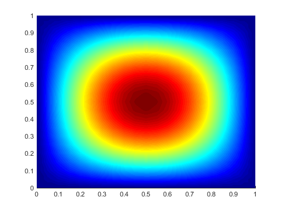
If you compile the program and run it, you compute a FE-approximation of the solution of the PDE. In the directory where you run the program you will find a MAT-file named "firstSolution.mat". If you use Matlab you can load this MAT-file and plot the solution entering the following instructions in your Matlab command line

> load firstSolution.mat
> patch(x(msh), y(msh), u(msh), 'edgecolor', 'none')
> colormap jet

This gives you the following visualization of the solution . Matlab output

You can visualize the vertexes and the edges of the mesh entering the following instructions in your Matlab command line

> hold on ; plot(x(vtxmsh), y(vtxmsh), 'ko') ; hold off

> hold on ; plot(x(edgemsh), y(edgemsh), 'k-') ; hold off

Complete Source Code

#include "hp2D.hh"
#include "concepts.hh"
 
using concepts::Real;
 
int main(int argc, char** argv) {
 
  // build a mesh of a unit square with edges of attribute 1
  concepts::Square mesh(1, 1, 1);
 
  // set homogeneous Dirichlet boundary conditions for every edge of attribute 1 (i.e. all edges) 
  concepts::BoundaryConditions bc;
  bc.add(concepts::Attribute(1),concepts::Boundary(concepts::Boundary::DIRICHLET));
 
  // build the finite element space V_2_5
  uint levelOfRefinement = 2;
  uint polynomialDegree = 6;
  hp2D::hpAdaptiveSpaceH1 space(mesh,levelOfRefinement,polynomialDegree,&bc);
  space.rebuild();
 
  // define the linear form f of the right hand side
  concepts::ParsedFormula<> f("((2*pi*pi+1)*sin(pi*x)*sin(pi*y))");
  hp2D::Riesz<Real> lform(f);
 
  // compute the vector for the finite element discretization
  concepts::Vector<Real> rhs(space, lform);
 
  // define the bilinear forms
  hp2D::Laplace<Real> la;
  hp2D::Identity<Real> id;
 
  // compute the mass and stiffness matrices
  concepts::SparseMatrix<Real> S(space, la);
  concepts::SparseMatrix<Real> M(space, id);
 
  // add mass matrix to stiffness matrix
  M.addInto(S, 1.);
 
  // compute the solution of the linear problem using the CG-method
  std::unique_ptr<concepts::Operator<Real> > solver(nullptr);
  solver.reset(new concepts::CG<Real>(S, 1e-12, 400));
  concepts::Vector<Real> sol(space);
  (*solver)(rhs, sol);
 
  // set integration points to be equidistant using trapezoidal rule
  hp2D::IntegrableQuad::factory().get()->setTensor(concepts::TRAPEZE, true, polynomialDegree);
  space.recomputeShapefunctions();
 
  // save graphical output of the solution in a MAT-file
  graphics::MatlabBinaryGraphics mbg(space, "firstSolution");
  mbg.addSolution(space, "u", sol);
 
  return 0;
}
 

howToGetStarted.cc

Introduction

Commented Program

Complete Source Code