elasticity2D_tutorial.cc

Contents

  1. Introduction
  2. Reduction to 2-dimensional elasticity
  3. Variational Formulation
  4. Commented Program
  5. Results
  6. Complete Source Code

Introduction

In this tutorial the implementation of linear elasticity problems in 2D is shown. We consider a thin plate with a hole at its centre. The plate is fixed at its left face and and there is some applied force on its right face. This is shown in the following figure. Sketch of problem 
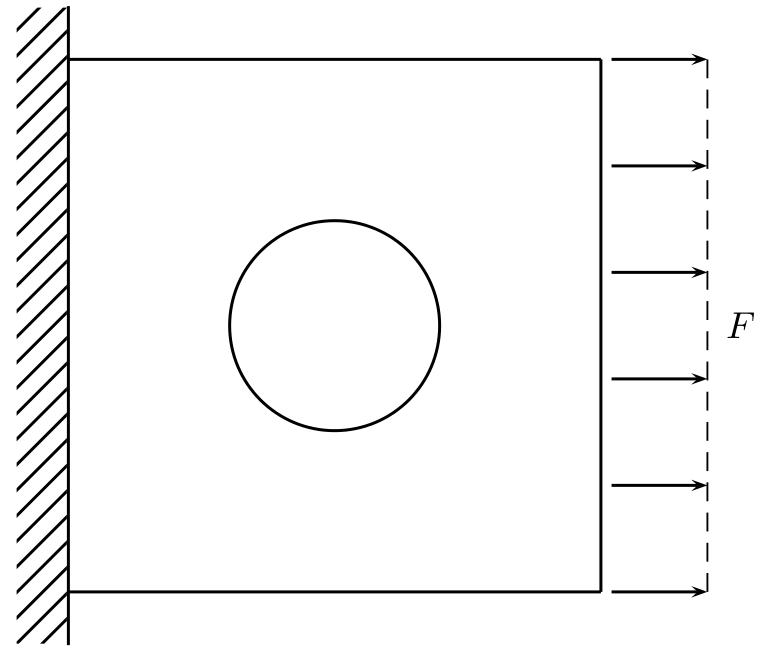
First we will give a short overview of the equations of linear elasticity in three dimensions and then reduce the problem to two dimensions.

The equation to be solved is

\[ - {\rm div} \:\sigma(u) = f \quad \text{in } \Omega, \]

for the unknown displacement $ u: \Omega \rightarrow \mathbb{R}^3 $ where $ \Omega \subseteq \mathbb{R}^3 $.
The applied body forces are described by the mapping $ f: \Omega \rightarrow \mathbb{R}^3 $, called the density of the applied body force per unit volume. The tensor $ \sigma(u) $ is the stress tensor, which will be described later.

On a subset $ \Gamma_0 \subseteq \partial\Omega $ the body is fixed and we get the homogenous Dirichlet boundary condition

\[ u = 0 \quad \text{on } \Gamma_0. \]

On the subset $ \Gamma_1 \subseteq \partial\Omega $ we have applied surface forces, which are given by a mapping $ g: \Gamma_1 \rightarrow \mathbb{R}^3 $
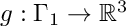
, called the density of the applied surface force per unit area. From that we get the boundary condition

\[ \sigma(u) n = g \quad \text{on } \Gamma_1, \]

where $ n $ is the unit outer normal vector along $ \Gamma_1 $.

The linear stress tensor is given by (also known as Hooke's Law)

\[ \sigma(u) = \lambda\; {\rm trace} (\varepsilon(u)) + 2\mu \varepsilon(u). \]

with the linear strain tensor

\[ \varepsilon_{ij}(u) = \frac{1}{2} (\partial_j u_i + \partial_i u_j ). \]

Reduction to 2-dimensional elasticity

For the reduction to a 2-dimensional problem there are two kinds of reduction techniques: the plane stress state and the plane strain state. The plane stress state is a good approximation for very thin bodies. In this case one can assume that all components of $ \sigma(u) $ connected to the $ x_3 $-direction vanish, i.e.

\[ \sigma_{i3}(u) = \sigma_{3i}(u) = 0 \quad i=1,2,3. \]

By throwing away the component of $ u $ in the $ x_3 $-direction and expressing $ \varepsilon_{33}(u) $ by $ \varepsilon_{11}(u) $ and $ \varepsilon_{22}(u) $, we can write the material law from the first section in the form

\[ \sigma^{\rm 2D} (u) = 2\mu \frac{\lambda}{\lambda+2\mu}\; {\rm trace}\left(\varepsilon^{\rm 2D}(u)\right) + 2\mu \varepsilon^{\rm 2D}(u). \]

For the plane strain state one can assume that all components of $ \varepsilon(u) $ connected to the $ x_3 $-direction vanish. Again by throwing away the component of $ u $ in the $ x_3 $-direction one can then write the material law in the form

\[ \sigma^{\rm 2D} (u) = \lambda\; {\rm trace}\left(\varepsilon^{\rm 2D}(u)\right) + 2\mu \varepsilon^{\rm 2D}(u). \]

Here we will use the plane stress state.

Variational Formulation

We choose

\[ V := \{ v \in H^1(\Omega)^2\,|\,\text{with } v = 0 \text{ on } \Gamma_0 \} \]

where now $ \Omega \subseteq \mathbb{R}^2 $. Then we have the bilinearform

\[ B(u,v) = \int_\Omega \sigma^{\rm 2D}(u):\varepsilon^{\rm 2D}(v) \;{\rm d}x \]

with $ u,v \in V $. Here we use for matrices $ A:B := \sum_{i,j=1}^n a_{ij}b_{ij} = {\rm trace}(A^T B) $.

Finally, the variational formulation is: Find $ u \in V $ such that

\[ 2\mu \frac{\lambda}{\lambda+2\mu} \int_\Omega {\rm div}(u){\rm div}(v) \;{\rm d}x + 2\mu \int_\Omega \varepsilon^{\rm 2D}(u): \varepsilon^{\rm 2D}(v) \;{\rm d}x = \int_\Omega f \cdot v \;{\rm d}x + \int_{\Gamma_1} g \cdot v \;{\rm d}s \quad \forall v \in V \]

in the case of the plane stress state and

\[ \lambda \int_\Omega {\rm div}(u){\rm div}(v) \;{\rm d}x + 2\mu \int_\Omega \varepsilon^{\rm 2D}(u): \varepsilon^{\rm 2D}(v) \;{\rm d}x = \int_\Omega f \cdot v \;{\rm d}x + \int_{\Gamma_1} g \cdot v \;{\rm d}s \quad \forall v \in V \]

in the case of the plane strain state. We will use this splitting of the bilinear form for computing the system matrix later.

Commented Program

First, systemfiles

#include <iostream>

and conceptfiles

#include "basics.hh"
#include "formula.hh"
#include "function.hh"
#include "geometry.hh"
#include "graphics.hh"
#include "hp2D.hh"
#include "hp1D.hh"
#include "operator.hh"
#include "space.hh"
#include "toolbox.hh"
#include "vectorial.hh"

are included. In this example we use a cig-file as input. This file is create with a Python script and contains geometry data, the densities of the applied forces, material constants and values for the h- and p-refinement. For using that cig-file as input, we write a method that first sets some default values and then reads the file.

void processInput(int argc, char** argv, concepts::InOutParameters& input)
{
input.addString("projname", "project");
input.addBool("plain_stress", 1);
input.addString("f1", "(0)");
input.addString("f2", "(0)");
input.addString("g1", "(1000000)");
input.addString("g2", "(0)");
input.addInt("dirichlet", 1);
input.addInt("neumann", 2);
input.addInt("delete", 11);
input.addInt("h", 3);
input.addInt("p", 2);
input.addInt("graphicpoints", 4);
concepts::ProcessParameter parameter(input);
if (!parameter.apply(argc, argv))
exit(1);
}

We first read the input data from the cig-file

int main(int argc, char *argv[]){
try {
processInput(argc, argv, input);

and save the material constants and the applied forces (each component is one function) for better access in some variables.

Then the mesh is generated and we write the mesh to an eps-file.

std::unique_ptr<concepts::Mesh2>
std::cout << "Mesh: " << *msh << std::endl;
graphics::drawMeshEPS( *msh, input.getString("projname") + "_mesh.eps", 100, 1.0, 100);

We load the attribute of the edges with the Dirichlet boundary condition from the input file and set the boundary condition for all edges with this attribute.

Now we first create a scalar space for the several components of the solution and save it again in an eps-file.

hp2D::hpAdaptiveSpaceH1 spc(*msh, input.getInt("h"), input.getInt("p"), &bc);
spc.rebuild();
std::cout << "spc = " << spc << std::endl;
graphics::drawMeshEPS(spc, input.getString("projname") + "_space.eps", 100, 1.0, 4);

We can then put this space into the components of the vectorial space.

const uint vdim = 2;
vspc.put(spc);
vspc.put(spc);
vspc.rebuild();

We create a trace space for the Neumann boundary condition.

hp2D::TraceSpace tspc(spc, concepts::makeSet<uint>({attrib_neumann}));

Now, we can compute the system matrix, where we use the splitted form of the bilinear form as stated in the variational formulation of the problem.

concepts::SparseMatrix<concepts::Real> S(vspc.dim(), vspc.dim());
hp2D::setupDivDiv(divdiv_bf);
A.addInto(S, 2*mu*lambda / (lambda + 2*mu));
B.addInto(S,2*mu);

The right hand side vectors are computed from the applied volume and surface forces. We compute these vectors for each component of the forces and concatenate them to one vector for the vectorial system.

rhs.add(rhs1);
rhs.add(rhs2,1.0,spc.dim());
hp1D::Riesz<concepts::Real> traceLForm1(g1);
hp1D::Riesz<concepts::Real> traceLForm2(g2);
concepts::Vector<concepts::Real> rhsNeumann1(tspc, traceLForm1);
concepts::Vector<concepts::Real> rhsNeumann2(tspc, traceLForm2);
rhs.add(rhsNeumann1);
rhs.add(rhsNeumann2,1.0,tspc.dim());

We solve the system with a direct method provided by SuperLU.

#else
#endif
solver(rhs, sol);

For better access and post-processing we split the solution into the two parts $ u_1 $ and $ u_2 $.

Now we write the solution (the displacement) and the resulting strains and stresses to a matlab binary file. Before doing that we recompute the shape functions on equidistant points.

hp2D::IntegrableQuad::factory().get()->setTensor(concepts::TRAPEZE, true, input.getInt("graphicpoints"));
spc.recomputeShapefunctions();
graphics::MatlabElasticityGraphics(spc,input.getString("projname")+"_stress",
sol_u1, sol_u2, lambda, mu, true);

We compute the energy norm of the solution.

concepts::Real energy_norm = sol*rhs;
std::cout << "Energy norm: " << std::setprecision(16) << energy_norm << std::endl;

Finally, exceptions are caught and a return value is given back.
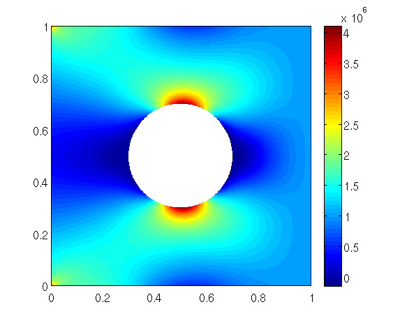
} catch (concepts::ExceptionBase& e) {
std::cout << e << std::endl;
return 1;
}

Results

For running this project we first have to create the cig file with the python script

python elasticity2D.py

With a symbolic link named bin to the directory containing the binaries, we can start the program with

bin/elasticity2D -f elasticity2D/elasticity2D.cig

The output of the program on the screen is then

Mesh: Import2dMeshGeneral(ncell = 4)
spc = hpAdaptiveSpaceH1(dim = 9359 (V:1071, E:4192, I:4096), nelm = 1024)
Assembling system matrix ...
done.
Systemmatrix:
SparseMatrix(18718x18718, HashedSparseMatrix: 918392 (0.262125%) entries bound.)
Assembling RHS ...
done.
solve system ...
done.
Energy norm: 7.480971032756906

The output of the solutions of the program is saved in a file called elasticity2D_stress.mat. For regarding the output (for example the stress $ \sigma_{11} $) in MATLAB we can type the following in the MATLAB command window

load elasticity2D_stress
patch(x(msh),y(msh),stress11(msh),'edgecolor','none')
axis image
colorbar

This creates the following image. Matlab output

Complete Source Code

Author
Philipp Kliewe, 2013
#include <iostream>
#include "basics.hh"
#include "formula.hh"
#include "function.hh"
#include "geometry.hh"
#include "graphics.hh"
#include "hp2D.hh"
#include "hp1D.hh"
#include "operator.hh"
#include "space.hh"
#include "toolbox.hh"
#include "vectorial.hh"
void processInput(int argc, char** argv, concepts::InOutParameters& input)
{
//set default values
input.addString("projname", "project");
input.addBool("plain_stress", 1);
input.addString("f1", "(0)");
input.addString("f2", "(0)");
input.addString("g1", "(1000000)");
input.addString("g2", "(0)");
input.addInt("dirichlet", 1);
input.addInt("neumann", 2);
input.addInt("delete", 11);
input.addInt("h", 3);
input.addInt("p", 2);
input.addInt("graphicpoints", 4);
// read arguments and Inputfiles
concepts::ProcessParameter parameter(input);
if (!parameter.apply(argc, argv))
exit(1);
}
int main(int argc, char *argv[]){
try {
#ifdef HAS_MPI
// Initialisation is necessary if parallel version of Mumps is compiled
MPI_Init(&argc, &argv);
#endif
// read CIG-file
processInput(argc, argv, input);
// read Lame-constants
const concepts::Real lambda = input.getDouble("lambda");
const concepts::Real mu = input.getDouble("mu");
// read formulas for the applied forces
// read and generate the mesh
std::unique_ptr<concepts::Mesh2>
std::cout << "Mesh: " << *msh << std::endl;
graphics::drawMeshEPS( *msh, input.getString("projname") + "_mesh.eps", 100, 1.0, 100);
// set Dirchlet boundary conditions
// Space
hp2D::hpAdaptiveSpaceH1 spc(*msh, input.getInt("h"), input.getInt("p"), &bc);
spc.rebuild();
std::cout << "spc = " << spc << std::endl;
graphics::drawMeshEPS(spc, input.getString("projname") + "_space.eps", 100, 1.0, 4);
// Vectorial Space
const uint vdim = 2;
vspc.put(spc);
vspc.put(spc);
vspc.rebuild();
// Trace Space for Neumann boundary condition
uint attrib_neumann = input.getInt("neumann");
hp2D::TraceSpace tspc(spc, concepts::makeSet<uint>({attrib_neumann}));
// Build system matrix
std::cout << "Assembling system matrix ..." << std::endl;
concepts::SparseMatrix<concepts::Real> S(vspc.dim(), vspc.dim());
hp2D::setupDivDiv(divdiv_bf);
A.addInto(S, 2*mu*lambda / (lambda + 2*mu));
B.addInto(S,2*mu);
std::cout << "done." << std::endl;
std::cout << "Systemmatrix:" << std::endl << S << std::endl;
// Build RHS vectors
std::cout << "Assembling RHS ..." << std::endl;
rhs.add(rhs1);
rhs.add(rhs2,1.0,spc.dim());
hp1D::Riesz<concepts::Real> traceLForm1(g1);
hp1D::Riesz<concepts::Real> traceLForm2(g2);
concepts::Vector<concepts::Real> rhsNeumann1(tspc, traceLForm1);
concepts::Vector<concepts::Real> rhsNeumann2(tspc, traceLForm2);
rhs.add(rhsNeumann1);
rhs.add(rhsNeumann2,1.0,tspc.dim());
std::cout << "done." << std::endl;
// Solve system
std::cout << "solve system ..." << std::endl;
#ifdef HAS_MUMPS
#else
#endif
solver(rhs, sol);
// split the solution into the components u1 and u2
concepts::Vector<concepts::Real> sol_u2(spc, (concepts::Real*)sol + spc.dim());
// plot the solution
hp2D::IntegrableQuad::factory().get()->setTensor(concepts::TRAPEZE, true, input.getInt("graphicpoints"));
spc.recomputeShapefunctions();
graphics::MatlabElasticityGraphics(spc,input.getString("projname")+"_stress",
sol_u1, sol_u2, lambda, mu, true);
std::cout << "done." << std::endl;
// compute energy norm
concepts::Real energy_norm = sol*rhs;
std::cout << "Energy norm: " << std::setprecision(16) << energy_norm << std::endl;
} catch (concepts::ExceptionBase& e) {
std::cout << e << std::endl;
return 1;
}
#ifdef HAS_MPI
MPI_Finalize();
#endif
return 0;
}
void hpAdaptiveSpaceH1(hp2D::hpAdaptiveSpaceH1 &spc, std::string str)
void setupLinStrainStrain(vectorial::BilinearForm< F, typename concepts::Realtype< F >::type > &bf, const concepts::ElementFormulaContainer< F, typename concepts::Realtype< F >::type > frm=concepts::ElementFormulaContainer< F, typename concepts::Realtype< F >::type >())
Builds the trace space of an FE space.
Definition: traces.hh:52
static std::unique_ptr< concepts::QuadRuleFactoryTensor2d > & factory()
Access to the quadrature rule, which is valid for all elements of this type (hp2D::IntegrableQuad).
Definition: quad.hh:145
@ TRAPEZE
Definition: defines.hh:13
Direct sparse solver for unsymmetric matrices.
Definition: superLU.hh:70
Vector valued space.
Definition: spaceTraits.hh:26
Import2dMeshGeneral * import2dMeshGeneralFromInput(const InOutParameters input, bool verbose=false)
Loads a mesh from a paramater list.
Base class for exceptions.
Definition: exceptions.hh:86
Vector valued bilinear form.
Definition: bf_advection.hh:38
MeshEPS< Real > drawMeshEPS(concepts::Mesh &msh, std::string filename, const Real scale=100, const Real greyscale=1.0, const unsigned int nPoints=2)
Trampoline function to create a MeshEPS.
void add(const Set< Attribute > &attrib, const Boundary &bcObject)
Adds a boundary condition with this attribute to the list of boundary conditions.
const concepts::Real norm(const concepts::Real &v)
Returns the square of a real value.
Definition: operations.hh:90
Holds parameters in hashes.
Definition: inputOutput.hh:75
double getDouble(const char *name) const
Returns a double from the hash of doubles.
Linear form on edges in nD.
Definition: linearForm.hh:67
int getInt(const char *name, const int value=INT_MAX) const
Returns an int from the hash of ints.
Class to describe an element of the boundary.
Definition: boundary.hh:35
void addString(const char *name, const char *value)
Adds a string to the hash of strings.
void addBool(const char *name, const int value)
Adds a bool to the hash of bools.
bool apply(int argc, char **argv)
Process the command line arguments.
void addInt(const char *name, const int value)
Adds an int to the hash of ints.
Linear form in 2D.
Definition: linearForm.hh:62
MUMPS : MUltifrontal Massively Parallel sparse direct Solver.
Definition: mumps.hh:72
std::string getString(const char *name, const char *value=0) const
Returns a string from the hash of strings.
Attributes for elements of the topology.
Definition: connector.hh:22
Reads command line.
Definition: inputParam.hh:81
double Real
Type normally used for a floating point number.
Definition: typedefs.hh:36
void setupDivDiv(vectorial::BilinearForm< F, typename concepts::Realtype< F >::type > &bf, const concepts::ElementFormulaContainer< F, typename concepts::Realtype< F >::type > frm=concepts::ElementFormulaContainer< F, typename concepts::Realtype< F >::type >())
Function to setup a bilinear form.
Page URL: http://wiki.math.ethz.ch/bin/view/Concepts/WebHome
21 August 2020
© 2020 Eidgenössische Technische Hochschule Zürich